Poisson mean scale invariant
Dongyue Xie
2019-11-11
Last updated: 2019-11-12
Checks: 7 0
Knit directory: SMF/
This reproducible R Markdown analysis was created with workflowr (version 1.5.0). The Checks tab describes the reproducibility checks that were applied when the results were created. The Past versions tab lists the development history.
Great! Since the R Markdown file has been committed to the Git repository, you know the exact version of the code that produced these results.
Great job! The global environment was empty. Objects defined in the global environment can affect the analysis in your R Markdown file in unknown ways. For reproduciblity it’s best to always run the code in an empty environment.
The command set.seed(20190719) was run prior to running the code in the R Markdown file. Setting a seed ensures that any results that rely on randomness, e.g. subsampling or permutations, are reproducible.
Great job! Recording the operating system, R version, and package versions is critical for reproducibility.
Nice! There were no cached chunks for this analysis, so you can be confident that you successfully produced the results during this run.
Great job! Using relative paths to the files within your workflowr project makes it easier to run your code on other machines.
Great! You are using Git for version control. Tracking code development and connecting the code version to the results is critical for reproducibility. The version displayed above was the version of the Git repository at the time these results were generated.
Note that you need to be careful to ensure that all relevant files for the analysis have been committed to Git prior to generating the results (you can use wflow_publish or wflow_git_commit). workflowr only checks the R Markdown file, but you know if there are other scripts or data files that it depends on. Below is the status of the Git repository when the results were generated:
Ignored files:
    Ignored:    .DS_Store
    Ignored:    .Rhistory
    Ignored:    .Rproj.user/
    Ignored:    analysis/.DS_Store
    Ignored:    data/.DS_Store

Untracked files:
    Untracked:  analysis/SMFrealdata.Rmd
    Untracked:  analysis/poissonmeanscle.Rmd
    Untracked:  data/external_data/

Unstaged changes:
    Modified:   analysis/poissonmean.Rmd
Note that any generated files, e.g. HTML, png, CSS, etc., are not included in this status report because it is ok for generated content to have uncommitted changes.
These are the previous versions of the R Markdown and HTML files. If you’ve configured a remote Git repository (see ?wflow_git_remote), click on the hyperlinks in the table below to view them.
| File | Version | Author | Date | Message |
|---|---|---|---|---|
| html | 80f97cf | Dongyue Xie | 2019-11-12 | Build site. |
| Rmd | 8b53d6c | Dongyue Xie | 2019-11-12 | wflow_publish(“analysis/poissonmean2.Rmd”) |
| html | 83f336c | Dongyue Xie | 2019-11-12 | Build site. |
| Rmd | 559b3e2 | Dongyue Xie | 2019-11-12 | wflow_publish(“analysis/poissonmean2.Rmd”) |
| html | 2bec0d4 | Dongyue Xie | 2019-11-12 | Build site. |
| Rmd | 9926eea | Dongyue Xie | 2019-11-12 | wflow_publish(“analysis/poissonmean2.Rmd”) |
Introduction
See if scale-invariant version could handle large scale case.
library(ebpm)
set.seed(12345)
pi0=0.8
lamda=c()
n=100
for(i in 1:100){
  idx = rbinom(1,1,pi0)
  if(idx){
    lamda[i] = rgamma(1,0.1,1)
  }else{
    lamda[i]=rgamma(1,50,1)
  }
}

lamda = sort(lamda)

hist(lamda,breaks =20)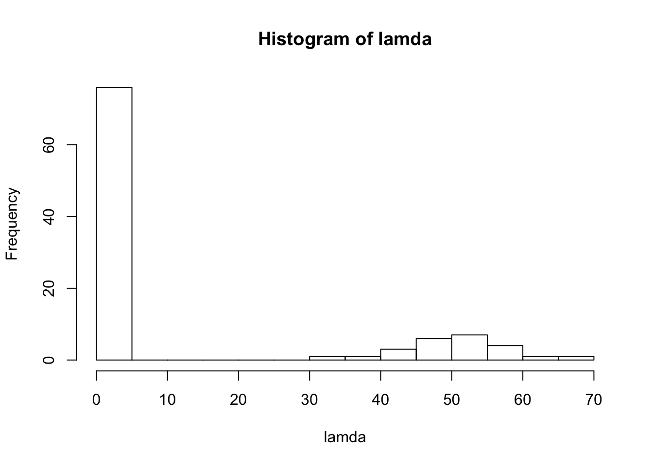
x = rpois(n,lamda)
s=1
fit = ebpm_gamma_mixture_single_scale(x,s)

plot(x/s,fit$posterior$mean,xlab = 'MLE',ylab = 'Posterior mean',pch=16)
abline(0,1)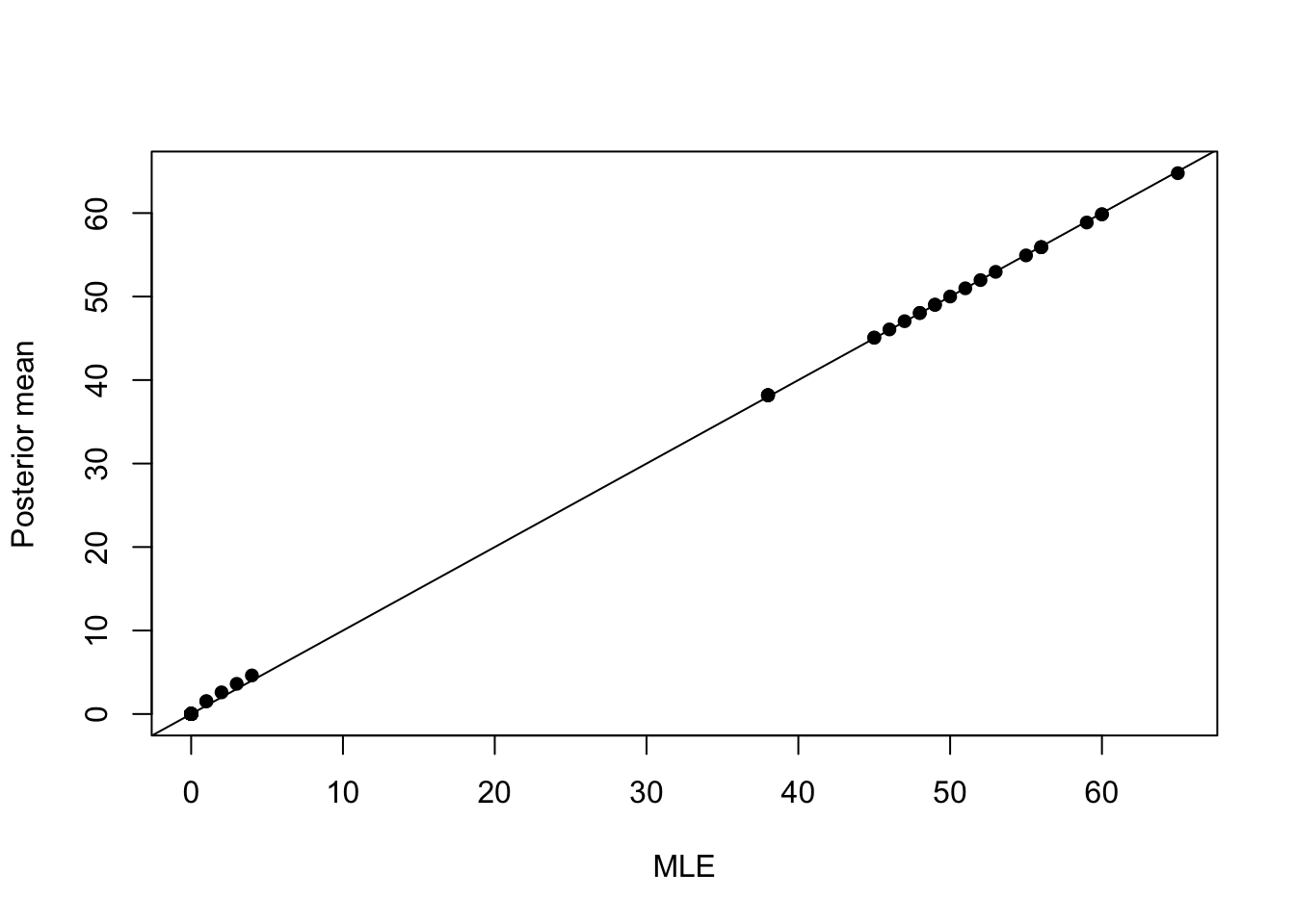
plot(x/s,col='grey80',pch=16)
lines(fit$posterior$mean,type='p',pch=3,col=2)
legend('topleft',c('MLE','Posterior mean'),col=c(1,2),pch=c(16,3))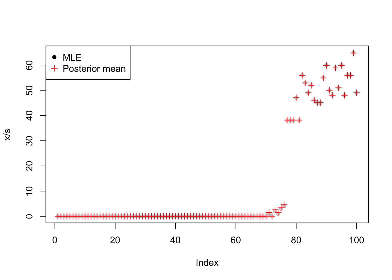
| Version | Author | Date |
|---|---|---|
| 83f336c | Dongyue Xie | 2019-11-12 |
No shrinkage estimate when \(x=0,1,2\).
How about \(\exp(E\log\lambda)\)?
plot((x/s),col='grey80',pch=16)
lines(exp(fit$posterior$mean_log),type='p',pch=3,col=2)
legend('topleft',c('MLE','exp(Posterior mean log)'),col=c(1,2),pch=c(16,3))
It shrinks \(E\log\lambda\) when \(x\) is large.
Look at estimated values from 70 to 80
(x/s)[70:80] [1] 0 1 0 2 1 3 4 38 38 38 47round(exp(fit$posterior$mean_log[70:80]),3) [1] 0.000 1.005 0.000 2.095 1.005 3.122 4.130 37.691 37.691 37.691
[11] 46.557Look at fitted prior
fit$fitted_g$pi
[1] 0.0000000 0.0000000 0.2311031 0.4836700 0.0000000 0.0000000 0.0000000
[8] 0.0000000 0.0000000 0.0000000 0.2852269 0.0000000 0.0000000
$shape
[1] 0.0007692308 0.0015384615 0.0030769231 0.0061538462 0.0123076923
[6] 0.0246153846 0.0492307692 0.0984615385 0.1969230769 0.3938461538
[11] 0.7876923077 1.5753846154 3.1507692308
$scale
[1] 65 65 65 65 65 65 65 65 65 65 65 65 65
attr(,"class")
[1] "gammamix"
attr(,"row.names")
[1] 1 2 3 4 5 6 7 8 9 10 11 12 13Let’s increase scale to \(s=100\).
set.seed(12345)
s = 100
x = rpois(n,s*lamda)
fit = ebpm_gamma_mixture_single_scale(x,s)

plot(x/s,fit$posterior$mean,xlab = 'MLE',ylab = 'Posterior mean',pch=16)
abline(0,1)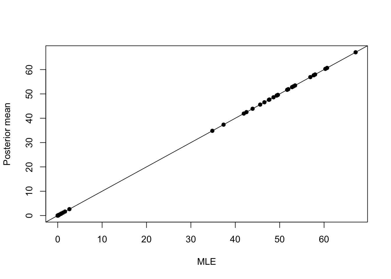
plot(x/s,col='grey80',pch=16)
lines(fit$posterior$mean,type='p',pch=3,col=2)
legend('topleft',c('MLE','Posterior mean'),col=c(1,2),pch=c(16,3))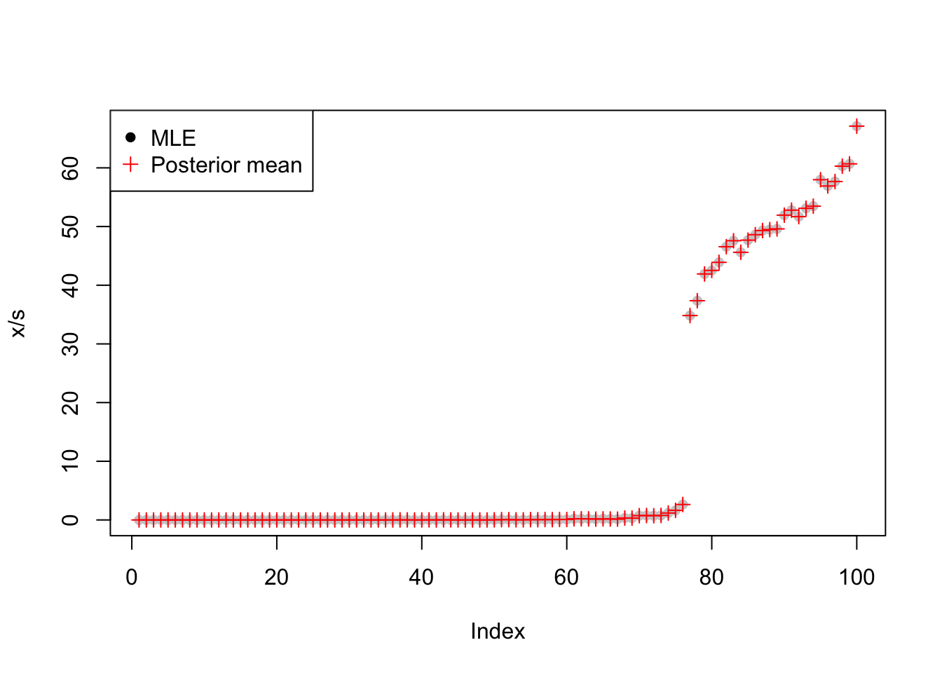
(x/s)[60][1] 0.08round(fit$posterior$mean[60],3)[1] 0.081No shrinkage estimate of \(\lambda\).
How about \(\exp(E\log\lambda)\)?
plot(x/s,exp(fit$posterior$mean_log),xlab = 'MLE',ylab = 'exp(Posterior mean log)',pch=16)
abline(0,1)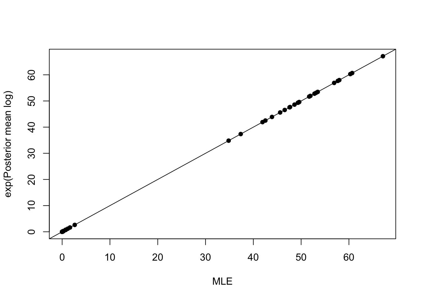
| Version | Author | Date |
|---|---|---|
| 83f336c | Dongyue Xie | 2019-11-12 |
plot(x/s,col='grey80',pch=16)
lines(exp(fit$posterior$mean_log),type='p',pch=3,col=2)
legend('topleft',c('MLE','exp(Posterior mean log)'),col=c(1,2),pch=c(16,3))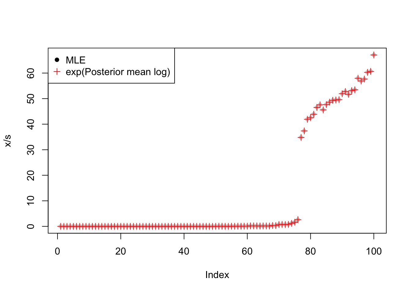
| Version | Author | Date |
|---|---|---|
| 83f336c | Dongyue Xie | 2019-11-12 |
(x/s)[60][1] 0.08round(exp(fit$posterior$mean_log)[60],3)[1] 0.076Some shrinkage, roughly \(2\%-5\%\) for some values. Maybe this is the reason why
Look at fitted prior
fit$fitted_g$pi
[1] 0.00000000 0.00000000 0.00000000 0.00000000 0.00000000 0.00000000
[7] 0.00000000 0.00000000 0.00000000 0.00000000 0.00000000 0.00000000
[13] 0.00000000 0.79795698 0.02294723 0.00000000 0.00000000 0.17909579
[19] 0.00000000 0.00000000
$shape
[1] 7.450454e-06 1.490091e-05 2.980182e-05 5.960364e-05 1.192073e-04
[6] 2.384145e-04 4.768291e-04 9.536582e-04 1.907316e-03 3.814633e-03
[11] 7.629265e-03 1.525853e-02 3.051706e-02 6.103412e-02 1.220682e-01
[16] 2.441365e-01 4.882730e-01 9.765460e-01 1.953092e+00 3.906184e+00
$scale
[1] 67.11 67.11 67.11 67.11 67.11 67.11 67.11 67.11 67.11 67.11 67.11
[12] 67.11 67.11 67.11 67.11 67.11 67.11 67.11 67.11 67.11
attr(,"class")
[1] "gammamix"
attr(,"row.names")
[1] 1 2 3 4 5 6 7 8 9 10 11 12 13 14 15 16 17 18 19 20
sessionInfo()R version 3.6.1 (2019-07-05)
Platform: x86_64-apple-darwin15.6.0 (64-bit)
Running under: macOS High Sierra 10.13.6
Matrix products: default
BLAS: /Library/Frameworks/R.framework/Versions/3.6/Resources/lib/libRblas.0.dylib
LAPACK: /Library/Frameworks/R.framework/Versions/3.6/Resources/lib/libRlapack.dylib
locale:
[1] en_US.UTF-8/en_US.UTF-8/en_US.UTF-8/C/en_US.UTF-8/en_US.UTF-8
attached base packages:
[1] stats graphics grDevices utils datasets methods base
other attached packages:
[1] ebpm_0.0.0.9004
loaded via a namespace (and not attached):
[1] workflowr_1.5.0 Rcpp_1.0.2 gtools_3.8.1 rprojroot_1.3-2
[5] digest_0.6.21 later_1.0.0 R6_2.4.0 backports_1.1.5
[9] git2r_0.26.1 magrittr_1.5 evaluate_0.14 stringi_1.4.3
[13] rlang_0.4.0 fs_1.3.1 promises_1.1.0 whisker_0.4
[17] rmarkdown_1.16 tools_3.6.1 stringr_1.4.0 glue_1.3.1
[21] mixsqp_0.1-97 httpuv_1.5.2 xfun_0.10 yaml_2.2.0
[25] compiler_3.6.1 htmltools_0.4.0 knitr_1.25