logo plots

One of the most basic applications of logo plots is to visualize the DNA sequence alignment(motif), which consists of four letters(A,C,G and T), corresponding to the four nucleotides(Adenine, Cytosine, Guanine, Thymine). The function logomaker() in Logolas provides the standard logo plots with the position weight matrix(PWM) as input. Here, we start with the same demo example provided in the seqLogo vignette.

library(Logolas)
mFile <- system.file("Exfiles/pwm1", package="seqLogo")
m <- read.table(mFile)
p <- seqLogo::makePWM(m)
color_profile <- list("type" = "per_row",
"col" = RColorBrewer::brewer.pal(dim(p@pwm)[1],name ="Spectral"))
logomaker(p@pwm,color_profile = color_profile, frame_width = 1,ic.scale = TRUE)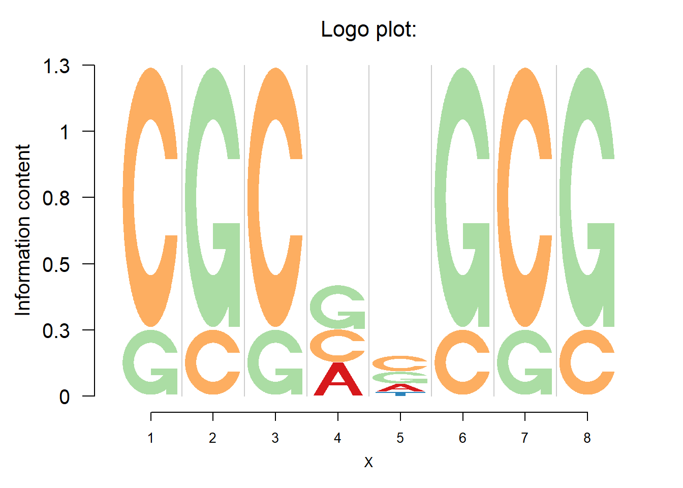

As a comparison, we present the logo plot of the same PWM from the package seqLogo.

seqLogo::seqLogo(p)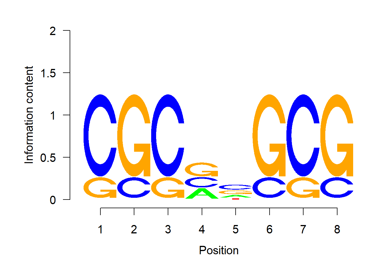

User could specify the color for each letter through the color_profile.

If ic.scale= TRUE, the heights of the bars at each position are determined by the Shannon entropy. The information content for position \(i\) is \(IC_i=-\Sigma_b p_{b}\times \log_2p_{b}-(-\Sigma_b q_{b,i}\times \log_2q_{b,i})\), where \(q_{b,i}\) is the relative frequency of base \(b\) at position \(i\) and \(p_{b}\) is the background probability of base \(b\). By default, the background probability of the each base is 0.25. So the information content at position \(i\) is \(IC_i=\Sigma_bq_{b,i}\times \log_2(q_{b,i}/0.25)\).

Logolas could also combine multiple plots into one overall graph. The figure below demonstrates the multiple panel plot as well as some variants of logo plots.

library(grid)

grid.newpage()
layout.rows <- 2
layout.cols <- 2
top.vp <- viewport(layout=grid.layout(layout.rows, layout.cols,
                                      widths=unit(rep(5,layout.cols), rep("null", 2)),
                                      heights=unit(rep(5,layout.rows), rep("null", 1))))
plot_reg <- vpList()
l <- 1
for(i in 1:layout.rows){
  for(j in 1:layout.cols){
    plot_reg[[l]] <- viewport(layout.pos.col = j, layout.pos.row = i, name = paste0("plotlogo", l))
    l <- l+1
  }
}


plot_tree <- vpTree(top.vp, plot_reg)

pushViewport(plot_tree)
#change the color of letters
#change the diverging palettes
color_profile1=list("type" = "per_row",
"col" = RColorBrewer::brewer.pal(dim(p@pwm)[1],name ="PiYG"))
seekViewport(paste0("plotlogo", 1))
logomaker(p@pwm,xlab = 'position',color_profile = color_profile1,
          frame_width = 1,
          newpage = FALSE,
          pop_name = 'Change color',
          control = list(viewport.margin.left = 5))

#change the y scale:
#if yscale_change = FALSE, then the height of y axis would be 2. 
seekViewport(paste0("plotlogo", 2))
logomaker(p@pwm,xlab = 'position',color_profile = color_profile,
          frame_width = 1,
          newpage = FALSE,
          pop_name = 'change y scale',
          yscale_change = FALSE,
          control = list(viewport.margin.left = 5))
#Normalize the height of bars to 1
seekViewport(paste0("plotlogo", 3))
logomaker(p@pwm,xlab = 'position',color_profile = color_profile,
          frame_width = 1,
          newpage = FALSE,
          ic.scale = FALSE,
          pop_name = 'Normalize the height',
          control = list(viewport.margin.left = 5))
#change the background probability
#And modify the title and the axis label 
seekViewport(paste0("plotlogo", 4))
logomaker(p@pwm,xlab = 'position',color_profile = color_profile,
          frame_width = 1,
          bg=c(0.32, 0.18, 0.2, 0.3),
          newpage = FALSE,
          pop_name = 'Change background prob',
          control = list(viewport.margin.left = 5))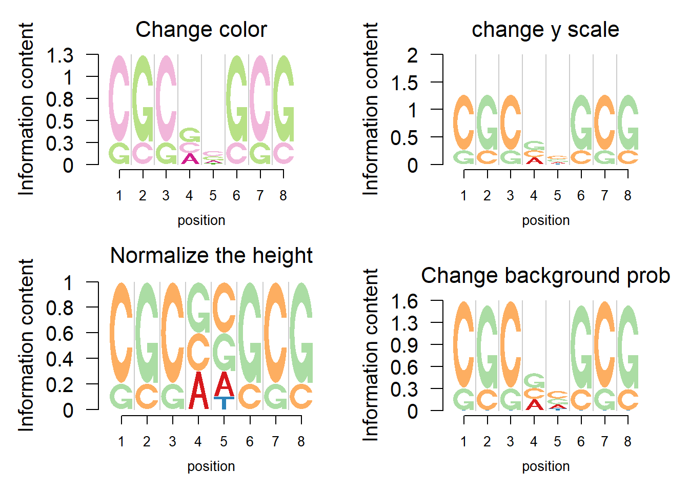

Choose the entropy

Besides the default Shannon entropy, logomaker could also get the information content using Renyi entropy. The information content at position \(i\) is \(IC_{i,\alpha}=\frac{1}{1-\alpha}\Sigma_b\log_2(q_{b,i}^\alpha-0.25^{1-\alpha})\). When \(\alpha\rightarrow1\), the limiting value of Renyi entropy is the Shannon entropy. The figure below shows the logo plot with different values of \(\alpha\).

grid.newpage()
layout.rows <- 1
layout.cols <- 2
top.vp <- viewport(layout=grid.layout(layout.rows, layout.cols,
                                      widths=unit(rep(6,layout.cols), rep("null", 2)),
                                      heights=unit(c(20,50), rep("lines", 2))))

plot_reg <- vpList()
l <- 1
for(i in 1:layout.rows){
  for(j in 1:layout.cols){
    plot_reg[[l]] <- viewport(layout.pos.col = j, layout.pos.row = i, name = paste0("plotlogo", l))
    l <- l+1
  }
}


plot_tree <- vpTree(top.vp, plot_reg)

pushViewport(plot_tree)
seekViewport(paste0("plotlogo", 1))
logomaker(p@pwm,xlab = 'position',color_profile = color_profile,
          frame_width = 1,
          newpage = FALSE,
          pop_name = 'Logo plot, Alpha=2',
          control = list(viewport.margin.left = 5,alpha=2))


seekViewport(paste0("plotlogo", 2))
logomaker(p@pwm,xlab = 'position',color_profile = color_profile,
          frame_width = 1,
          newpage = FALSE,
          pop_name = 'Logo plot, Alpha=0.2',
          control = list(viewport.margin.left = 5,alpha=0.2))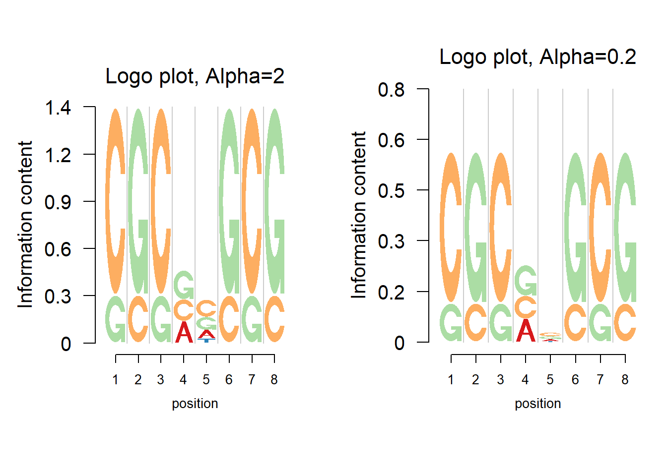

Negative logo plots

In the logo plot, the enrichment is highlighted while the depletion is usually overlooked. We hence propose the negative logo plot, in which the depletion is plotted down below the zero on y-axis so that we can find both strong positive and negative effects.

The nlogomaker function provides negative logo plot. And there are three different options of logo heights: information content, log probability and log-odds.

The negative logo plot actually shows the relative change of base frequencies. To achieve this, the median of base frequencies is subtracted at a position. For example, the relative frequencies at a position is \(P=(0.7,0.15,0.15,0)\); subtracted by the median, it becomes \(P_{neg}=(0.55,0,0,-0.15)\). Then the total heights are allocated to the positive and negative parts and further allocated to each base, based on \(P_{neg}\).

Below we show the negative logo plot using log and log-odds heights for the same example as above.

grid.newpage()
layout.rows <- 1
layout.cols <- 2
top.vp <- viewport(layout=grid.layout(layout.rows, layout.cols,
                                      widths=unit(rep(6,layout.cols), rep("null", 2)),
                                      heights=unit(c(20,50), rep("lines", 2))))

plot_reg <- vpList()
l <- 1
for(i in 1:layout.rows){
  for(j in 1:layout.cols){
    plot_reg[[l]] <- viewport(layout.pos.col = j, layout.pos.row = i, name = paste0("plotlogo", l))
    l <- l+1
  }
}


plot_tree <- vpTree(top.vp, plot_reg)

pushViewport(plot_tree)
seekViewport(paste0("plotlogo", 1))
nlogomaker(p@pwm,logoheight = 'log',color_profile = color_profile,frame_width = 1,newpage = FALSE)


seekViewport(paste0("plotlogo", 2))
nlogomaker(p@pwm,logoheight = 'log_odds',color_profile = color_profile,frame_width = 1,newpage = FALSE)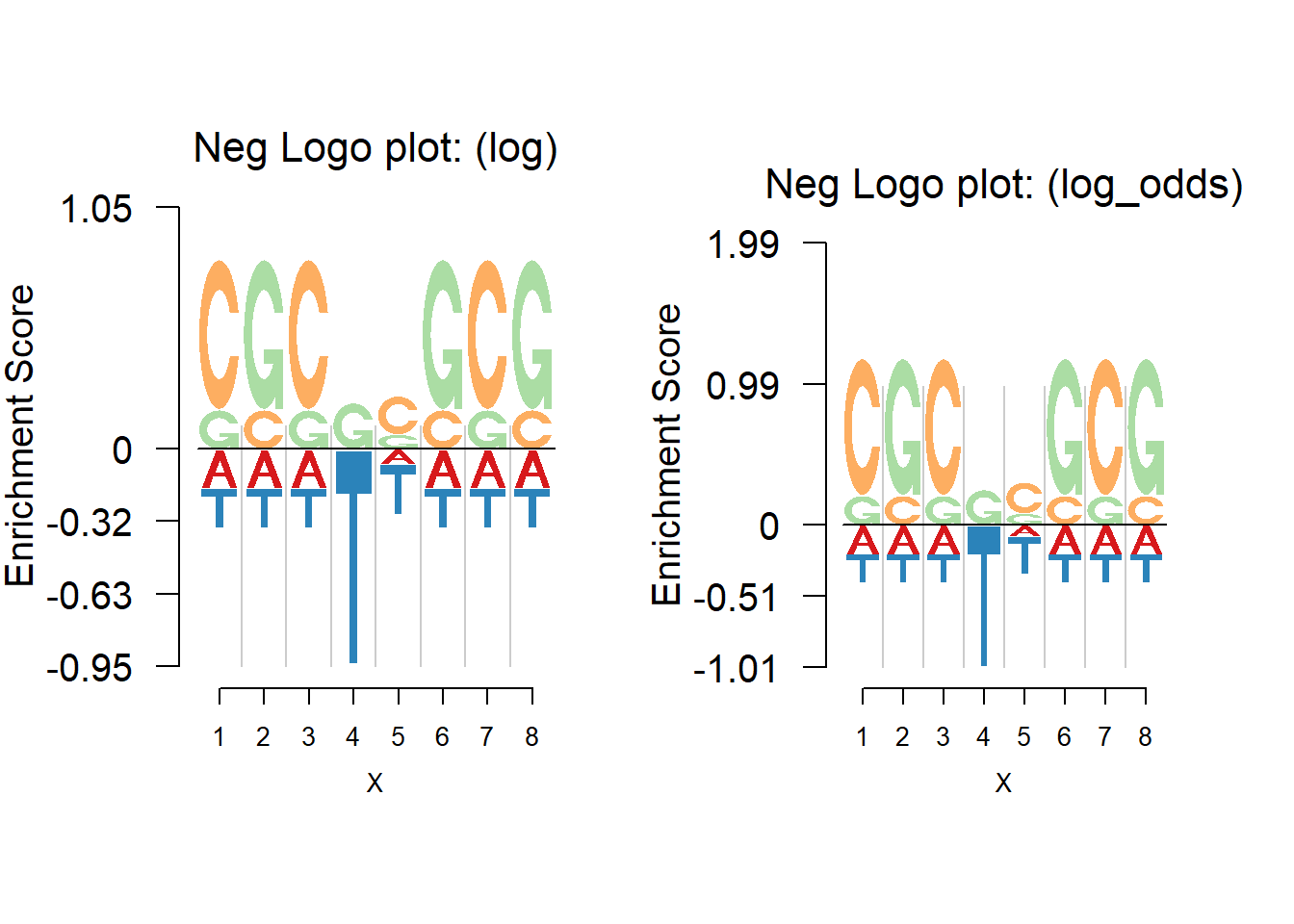

As seen from the above figures, the negative logo plot presents both the enrichment and depletion. For example, there is an obvious depletion of T at the position 4. It may be considered that the transcription factor(TF) would find both enrichment and depletion to decide whether to bind. For example, at position 4, the depletion of T probably means the TF dislikes T at that position.

Depletion weights

Logolas further allow users to customize the weight of depletion. As the depletion weight increasing, the depletion would look more prominent. The default depletion weight is 0.5 and comparisons of different depletion weights are shown below. The weights chosen are 0.1,0.3,0.5(default),1.

grid.newpage()
layout.rows <- 2
layout.cols <- 2
top.vp <- viewport(layout=grid.layout(layout.rows, layout.cols,
                                      widths=unit(rep(5,layout.cols), rep("null", 2)),
                                      heights=unit(rep(5,layout.rows), rep("null", 1))))
plot_reg <- vpList()
l <- 1
for(i in 1:layout.rows){
  for(j in 1:layout.cols){
    plot_reg[[l]] <- viewport(layout.pos.col = j, layout.pos.row = i, name = paste0("plotlogo", l))
    l <- l+1
  }
}


plot_tree <- vpTree(top.vp, plot_reg)

pushViewport(plot_tree)
seekViewport(paste0("plotlogo", 1))
nlogomaker(p@pwm,
           logoheight = 'log_odds',
           color_profile = color_profile,
           frame_width = 1,
           newpage = FALSE,
           pop_name = 'Weight=0.1',
           control = list(depletion_weight=0.1))


seekViewport(paste0("plotlogo", 2))
nlogomaker(p@pwm,
           logoheight = 'log_odds',
           color_profile = color_profile,
           frame_width = 1,
           newpage = FALSE,
            pop_name = 'Weight=0.3',
           control = list(depletion_weight=0.3))

seekViewport(paste0("plotlogo", 3))
nlogomaker(p@pwm,
           logoheight = 'log_odds',
           color_profile = color_profile,
           frame_width = 1,
           newpage = FALSE,
            pop_name = 'Weight=0.5',
           control = list(depletion_weight=0.5))

seekViewport(paste0("plotlogo", 4))
nlogomaker(p@pwm,
           logoheight = 'log_odds',
           color_profile = color_profile,
           frame_width = 1,
           newpage = FALSE,
            pop_name = 'Weight=1',
           control = list(depletion_weight=1))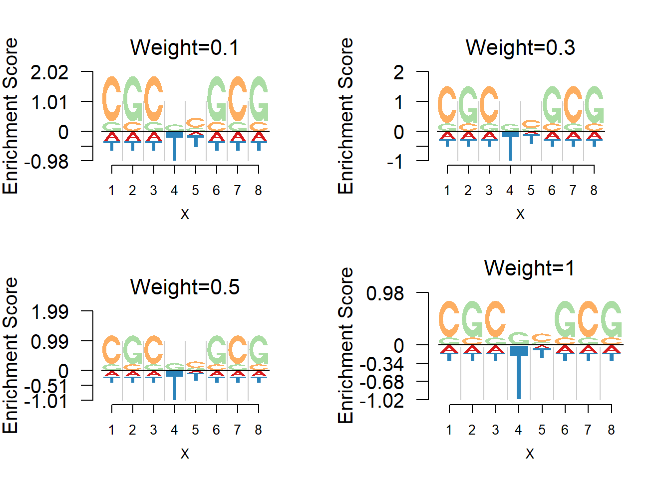

Border and fill

User could customize the border and fill of the logos. For example, the user may choose to fill the enrichment while only show the border of depletion. The figure below shows the various option on making the logos.

grid.newpage()
layout.rows <- 2
layout.cols <- 2
top.vp <- viewport(layout=grid.layout(layout.rows, layout.cols,
                                      widths=unit(rep(5,layout.cols), rep("null", 2)),
                                      heights=unit(rep(5,layout.rows), rep("null", 1))))

plot_reg <- vpList()
l <- 1
for(i in 1:layout.rows){
  for(j in 1:layout.cols){
    plot_reg[[l]] <- viewport(layout.pos.col = j, layout.pos.row = i, name = paste0("plotlogo", l))
    l <- l+1
  }
}


plot_tree <- vpTree(top.vp, plot_reg)

pushViewport(plot_tree)

seekViewport(paste0("plotlogo", 1))
nlogomaker(p@pwm,xlab = 'position',logoheight = "log",
           color_profile = color_profile,
           bg = c(0.25, 0.25, 0.25, 0.25),
           frame_width = 1,
           control = list(tofill_pos = TRUE, tofill_neg=FALSE,
                          logscale = 0.2, quant = 0.5,
                          depletion_weight = 0.5),
           newpage = FALSE)

seekViewport(paste0("plotlogo", 2))
nlogomaker(p@pwm,xlab = 'position',logoheight = "log",
           color_profile = color_profile,
           bg = c(0.25, 0.25, 0.25, 0.25),
           frame_width = 1,
           control = list(tofill_pos = FALSE, tofill_neg=TRUE,
                          logscale = 0.2, quant = 0.5,
                          depletion_weight = 0.5),
           newpage = FALSE)

seekViewport(paste0("plotlogo", 3))
nlogomaker(p@pwm,xlab = 'position',logoheight = "log",
           color_profile = color_profile,
           bg = c(0.25, 0.25, 0.25, 0.25),
           frame_width = 1,
           control = list(tofill_pos = TRUE, tofill_neg=TRUE,
                          logscale = 0.2, quant = 0.5,
                          depletion_weight = 0.5),
           newpage = FALSE)

seekViewport(paste0("plotlogo", 4))
nlogomaker(p@pwm,xlab = 'position',logoheight = "log",
           color_profile = color_profile,
           bg = c(0.25, 0.25, 0.25, 0.25),
           frame_width = 1,
           control = list(tofill_pos = FALSE, tofill_neg=FALSE,
                          logscale = 0.2, quant = 0.5,
                          depletion_weight = 0.5),
           newpage = FALSE)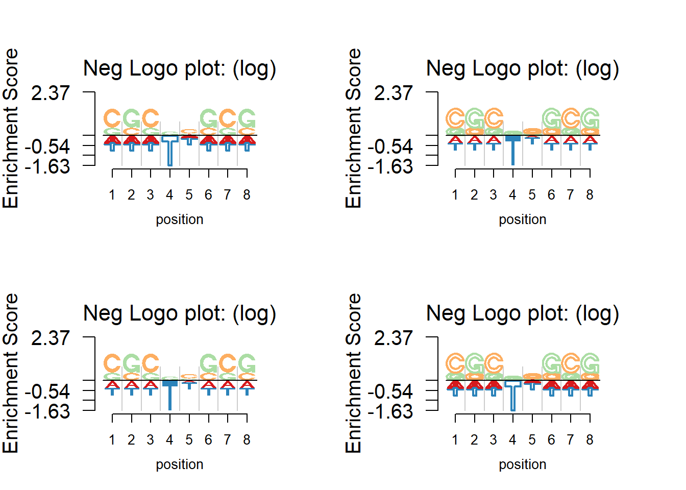

Session information

sessionInfo()

R version 3.4.0 (2017-04-21)
Platform: x86_64-w64-mingw32/x64 (64-bit)
Running under: Windows 10 x64 (build 15063)

Matrix products: default

locale:
[1] LC_COLLATE=English_United States.1252 
[2] LC_CTYPE=English_United States.1252   
[3] LC_MONETARY=English_United States.1252
[4] LC_NUMERIC=C                          
[5] LC_TIME=English_United States.1252    

attached base packages:
[1] grid      stats     graphics  grDevices utils     datasets  methods  
[8] base     

other attached packages:
[1] Logolas_1.1.2

loaded via a namespace (and not attached):
 [1] Rcpp_0.12.12       digest_0.6.12      rprojroot_1.2     
 [4] backports_1.0.5    stats4_3.4.0       git2r_0.18.0      
 [7] magrittr_1.5       evaluate_0.10      stringi_1.1.5     
[10] rmarkdown_1.6      RColorBrewer_1.1-2 tools_3.4.0       
[13] stringr_1.2.0      yaml_2.1.14        compiler_3.4.0    
[16] seqLogo_1.42.0     htmltools_0.3.5    knitr_1.15.1