Dirichlet adaptive shrinkage
Dongyue Xie
2017-08-26
Last updated: 2017-08-29
Code version: 8d27e6d
Logo plot is based on the position weight matrix(PWM), which is transformed from the position frequency matrix(PFM). PFM consists of the counts for each base at each position. This is a typical example of compositional data, which is used to describe the constituents of discrete sample space.
Suppose for a specific position of a TFBS, the compositional data is \[ (A, C, G, T) : = (6, 1, 2, 1) \] and one another case is \[ (A, C, G, T) : = (600, 100, 200, 100). \] And the background probability is assumed to be equal for the four bases. If we transform the counts data into PWM by using the sample proportion, then the estimated proportions for the four bases are the same in both cases. However, in the second case, we have total 1000 samples while only 10 samples in the first case. Hence, we would consider to shrink the estimates to the background probability more strongly in the first case than that in the second case, for the reason that the force of data is stronger in the second scenarios.
Model formulation
To address these questions, we propose Dirichlet adaptive shrinkage(dash) for compositional data. Assume that there are \(L\) constituents in the compositional mix. \(L\) equals \(4\) (corresponding to A,C, G and T bases) for the transcription factor data and \(20\) corresponding to the amino acids for the protein sequence data.
Suppose there are \(L\) categories and \(n\) compositional samples. Here, \(n\) represents the number of positions for a TF. We model these compositional counts vectors as follows
\[ (c_{n1}, c_{n2}, \cdots, c_{nL}) \sim Mult \left ( c_{n+} : p_{n1}, p_{n2}, \cdots, p_{nL} \right ) \]
where \(c_{n+}\) is the total frequency of the different constituents of the compositional data observed for the \(n\) th base. \(p_{nl}\) here represents the compositional probabilities such that
\[ p_{nl} >= 0 \hspace {1 cm} \sum_{l=1}^{L} p_{nl} = 1 \]
We then choose the Dirichlet prior distribution on the \((p_{n1}, p_{n2}, \cdots, p_{nL})\). In order to achieve the adaptive shrinkage property, we assume a mixture of known Dirichlet priors, each having mean same as the background mean but with varying amounts of concentration, along with unknown mixture proportions to be estimated from the data. \[ \left ( p_{n1}, p_{n2}, \cdots, p_{nL} \right ) : = \sum_{k=1}^{K} \pi_{k} Dir \left (\alpha_{k} \mu_{k1}, \alpha_{k} \mu_{k2}, \cdots, \alpha_{k} \mu_{kL} \right ) \hspace {1 cm} \alpha_{k} > 0 \hspace{1 cm} \sum_{l=1}^{L} \mu_{kl} = 1 \] We assume a prior of \(\pi_{k}\) to be Dirichlet
\[ f(\pi) : = \prod_{k=1}^{K} {\pi_{k}}^{\lambda_{k}-1} \]
Default parameters
We choose a default set of \(\alpha_{k}\) to be \((Inf, 100, 50, 20, 10, 2, 1, 0.1, 0.01)\). In this case \(\alpha_{k}=Inf\) corresponds essentially to point mass at the prior means, and then the subsequent choices of \(\alpha_{k}\) have lower degree of concentration. $_{k} = $ corresponds to the most uniform scenario, whereas \(\alpha_{k} < 1\) correspond to cases with probability masses at the edges of the simplex but with the mean at the prior mean. These components would help to direct the points close to the corners towards the corners and away from the center, resulting in clearer separation of the points closer to the mean with the ones away from it.
We choose the prior amount of shrinkage of \(\pi_{k}\), namely \(\lambda_{k}\) to be \(\left( 10, 1, 1, 1, \cdots, 1 \right )\).
Dash examples
We apply dash to PFMs with small, medium and high total frequencies(\(c_{n+}\)). The total frequencies in the three cases are 5,20 and 114. Firstly, the logo plots are compared and then negative logo plot.
Logo plots:
library(Logolas)
library(grid)
library(dash)
pfm1=cbind(c(1,2,1,1),c(0,0,5,0),c(0,3,1,1),c(0,5,0,0),c(0,3,0,2),c(0,0,5,0),c(2,1,2,0),c(0,0,5,0),c(1,1,0,3))
pfm2=cbind(c(1,9,5,5),c(1,16,2,1),c(1,1,18,0),c(1,0,2,17),c(18,1,0,1),c(1,18,0,0),c(1,2,16,1),c(6,4,7,3),c(2,12,1,5),c(8,5,5,2))
pfm3=cbind(c(31,8,46,29),c(1,2,25,86),c(12,34,11,57),c(3,1,106,4),c(1,110,1,2),c(3,1,109,1),c(0,3,1,110),c(0,0,114,0),c(33,57,6,18))
rownames(pfm1)=c('A','C','G','T')
colnames(pfm1)=1:ncol(pfm1)
rownames(pfm2)=c('A','C','G','T')
colnames(pfm2)=1:ncol(pfm2)
rownames(pfm3)=c('A','C','G','T')
colnames(pfm3)=1:ncol(pfm3)

color_profile = list("type" = "per_row",
                     "col" = RColorBrewer::brewer.pal(4,name ="Spectral"))

grid.newpage()
layout.rows <- 3
layout.cols <- 2
top.vp <- viewport(layout=grid.layout(layout.rows,layout.cols, widths=unit(rep(2,layout.cols), rep("null",layout.cols)),heights=unit(rep(2,1), rep("null",1))))

plot_reg <- vpList()
l <- 1
for(i in 1:layout.rows){
  for(j in 1:layout.cols){
    plot_reg[[l]] <- viewport(layout.pos.col = j, layout.pos.row = i, name = paste0("plotlogo", l))
    l <- l+1
  }
}


plot_tree <- vpTree(top.vp, plot_reg)

pushViewport(plot_tree)
seekViewport(paste0("plotlogo", 1))
logomaker(pfm1,
          color_profile = color_profile,
          frame_width = 1,
          newpage = F,
          yscale_change = F,
          pop_name = 'low freq')
seekViewport(paste0('plotlogo',2))
pfm1dash=t(dash(t(pfm1),optmethod = 'mixEM')$posmean)
rownames(pfm1dash)=c('A','C','G','T')
colnames(pfm1dash)=1:ncol(pfm1)
logomaker(pfm1dash,
          color_profile = color_profile,
          frame_width = 1,
          newpage=F,
          yscale_change = F,
          pop_name = 'low freq, dash')

seekViewport(paste0("plotlogo", 3))
logomaker(pfm2,
          color_profile = color_profile,
          frame_width = 1,
          newpage = F,
          yscale_change = F,
          pop_name = 'medium freq')
seekViewport(paste0('plotlogo',4))
pfm2dash=t(dash(t(pfm2),optmethod = 'mixEM')$posmean)
rownames(pfm2dash)=c('A','C','G','T')
colnames(pfm2dash)=1:ncol(pfm2)
logomaker(pfm2dash,
          color_profile = color_profile,
          frame_width = 1,
          newpage=F,
          yscale_change = F,
          pop_name = 'medium freq, dash')

seekViewport(paste0("plotlogo", 5))
logomaker(pfm3,
          color_profile = color_profile,
          frame_width = 1,
          newpage = F,
          yscale_change = F,
          pop_name = 'high freq')
seekViewport(paste0('plotlogo',6))
pfm3dash=t(dash(t(pfm3),optmethod = 'mixEM')$posmean)
rownames(pfm3dash)=c('A','C','G','T')
colnames(pfm3dash)=1:ncol(pfm3)
logomaker(pfm3dash,
          color_profile = color_profile,
          frame_width = 1,
          newpage=F,
          yscale_change = F,
          pop_name = 'high freq, dash')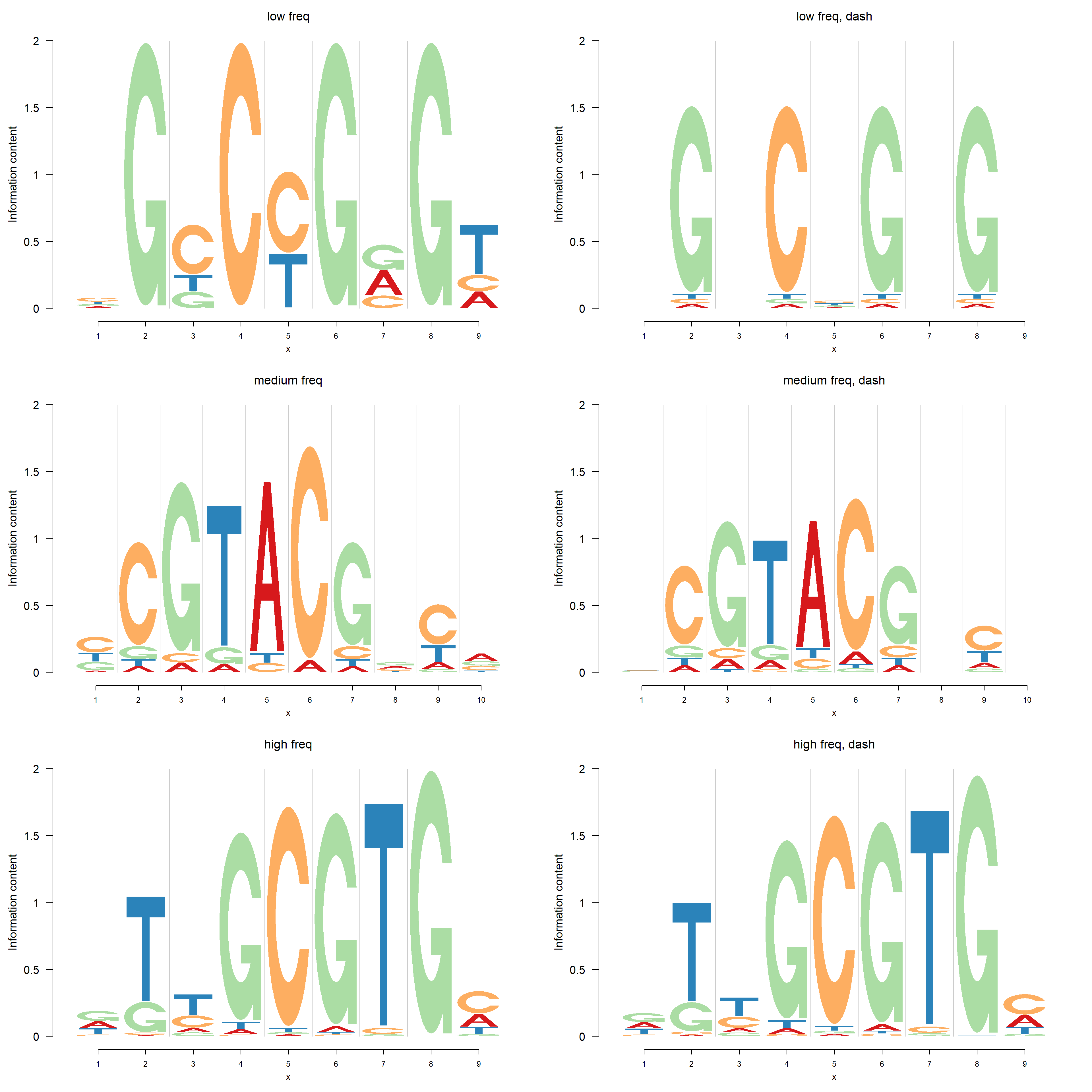
Negative logo plots:
grid.newpage()
layout.rows <- 3
layout.cols <- 2
top.vp <- viewport(layout=grid.layout(layout.rows,layout.cols, widths=unit(rep(2,layout.cols), rep("null",layout.cols)),heights=unit(rep(2,1), rep("null",1))))

plot_reg <- vpList()
l <- 1
for(i in 1:layout.rows){
  for(j in 1:layout.cols){
    plot_reg[[l]] <- viewport(layout.pos.col = j, layout.pos.row = i, name = paste0("plotlogo", l))
    l <- l+1
  }
}


plot_tree <- vpTree(top.vp, plot_reg)

pushViewport(plot_tree)
seekViewport(paste0("plotlogo", 1))
nlogomaker(pfm1,
           logoheight = 'log_odds',
          color_profile = color_profile,
          frame_width = 1,
          newpage = F,
          ylimit = 2.8,
          pop_name = 'low freq')

seekViewport(paste0('plotlogo',2))
pfm1dash=t(dash(t(pfm1),optmethod = 'mixEM')$posmean)
rownames(pfm1dash)=c('A','C','G','T')
colnames(pfm1dash)=1:ncol(pfm1)
nlogomaker(pfm1dash,
           logoheight = 'log_odds',
          color_profile = color_profile,
          frame_width = 1,
          newpage=F,
          ylimit = 2.5,
          pop_name = 'low freq, dash')

seekViewport(paste0("plotlogo", 3))
nlogomaker(pfm2,
           logoheight = 'log_odds',
          color_profile = color_profile,
          frame_width = 1,
          newpage = F,
          ylimit = 2.5,
          pop_name = 'medium freq')
seekViewport(paste0('plotlogo',4))
pfm2dash=t(dash(t(pfm2),optmethod = 'mixEM')$posmean)
rownames(pfm2dash)=c('A','C','G','T')
colnames(pfm2dash)=1:ncol(pfm2)
nlogomaker(pfm2dash,
          color_profile = color_profile,
          logoheight = 'log_odds',
          frame_width = 1,
          newpage=F,
          ylimit = 2.5,
          pop_name = 'medium freq, dash')

seekViewport(paste0("plotlogo", 5))
nlogomaker(pfm3,
           logoheight = 'log_odds',
          color_profile = color_profile,
          frame_width = 1,
          newpage = F,
          ylimit = 2.5,
          pop_name = 'high freq')
seekViewport(paste0('plotlogo',6))
pfm3dash=t(dash(t(pfm3),optmethod = 'mixEM')$posmean)
rownames(pfm3dash)=c('A','C','G','T')
colnames(pfm3dash)=1:ncol(pfm3)
nlogomaker(pfm3dash,
           logoheight = 'log_odds',
          color_profile = color_profile,
          frame_width = 1,
          newpage=F,
          ylimit = 2.5,
          pop_name = 'high freq, dash')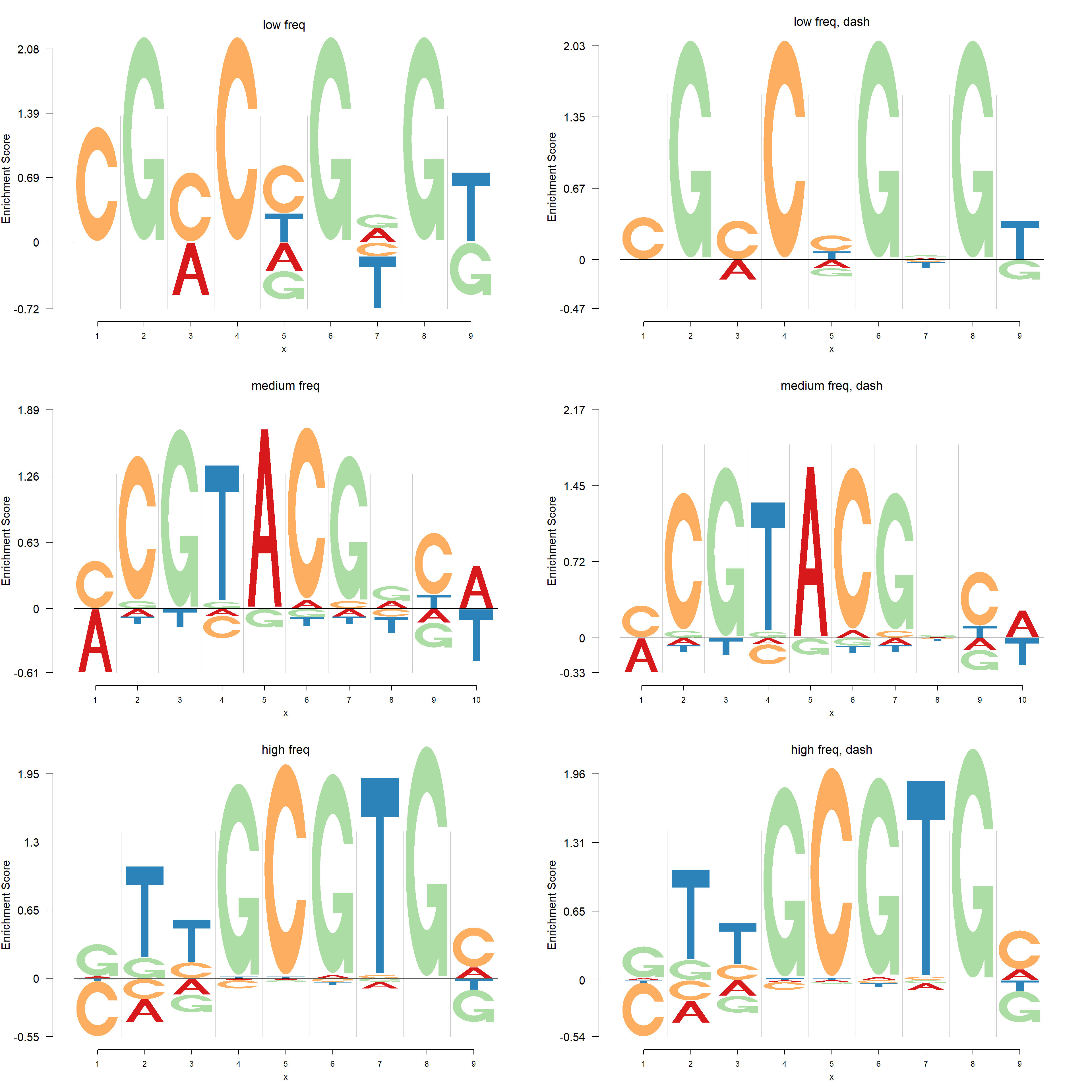
The default background probability is uniform for each compositional class. User could also specify the background probability in the functions including dash,logomaker,nlogomaker.
Here, we present the comparisons of logo plots and negative logo plots from 4 different PWMs of one PFM generated in the following way:
| 1 | 2 |
|---|---|
| same bg, no dash | same bg, dash |
| varying bg, no dash | varying bg, dash |
Logo plots:
bg=c(0.3141, 0.1859, 0.1859, 0.3141)
grid.newpage()
layout.rows <- 2
layout.cols <- 2
top.vp <- viewport(layout=grid.layout(layout.rows,layout.cols, widths=unit(rep(2,layout.cols), rep("null",layout.cols)),heights=unit(rep(2,1), rep("null",1))))

plot_reg <- vpList()
l <- 1
for(i in 1:layout.rows){
  for(j in 1:layout.cols){
    plot_reg[[l]] <- viewport(layout.pos.col = j, layout.pos.row = i, name = paste0("plotlogo", l))
    l <- l+1
  }
}


plot_tree <- vpTree(top.vp, plot_reg)

pushViewport(plot_tree)
seekViewport(paste0("plotlogo", 1))
logomaker(pfm2,
          color_profile = color_profile,
          frame_width = 1,
          newpage = F,
          yscale_change = F,
          pop_name = 'same bg, no dash')

seekViewport(paste0("plotlogo", 2))
logomaker(pfm2dash,
          color_profile = color_profile,
          frame_width = 1,
          newpage = F,
          yscale_change = F,
          pop_name = 'same bg, dash')


seekViewport(paste0("plotlogo", 3))
logomaker(pfm2,
          bg=bg,
          color_profile = color_profile,
          frame_width = 1,
          newpage = F,
          yscale_change = F,
          pop_name = 'varying bg, no dash')

pfm2dashbg=t(dash(t(pfm2),optmethod = 'mixEM',mode = bg)$posmean)
rownames(pfm2dashbg)=c('A','C','G','T')
colnames(pfm2dashbg)=1:ncol(pfm2)

seekViewport(paste0("plotlogo", 4))
logomaker(pfm2dashbg,
          bg=bg,
          color_profile = color_profile,
          frame_width = 1,
          newpage = F,
          yscale_change = F,
          pop_name = 'varying bg, dash')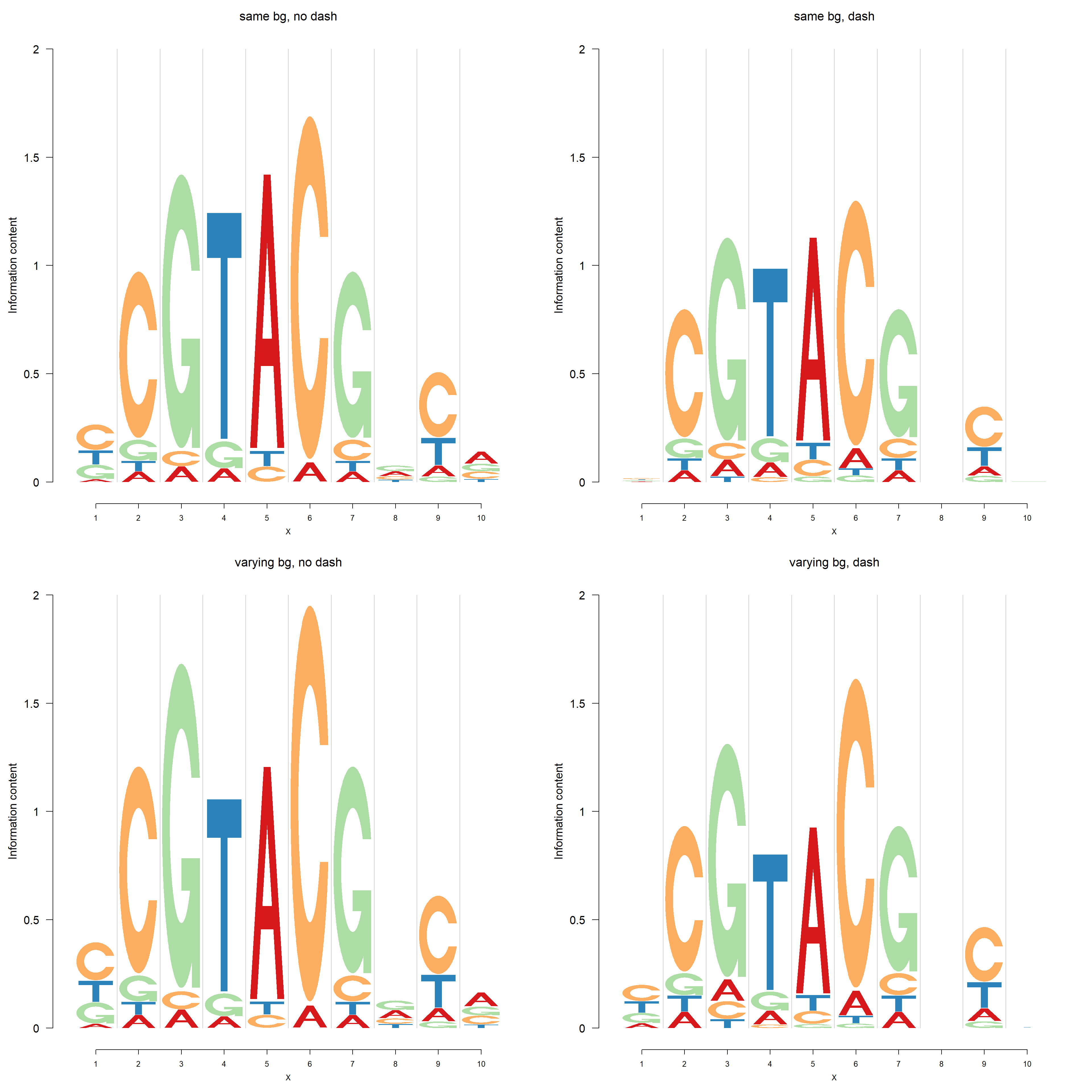
Negative logo plots:
grid.newpage()
layout.rows <- 2
layout.cols <- 2
top.vp <- viewport(layout=grid.layout(layout.rows,layout.cols, widths=unit(rep(2,layout.cols), rep("null",layout.cols)),heights=unit(rep(2,1), rep("null",1))))

plot_reg <- vpList()
l <- 1
for(i in 1:layout.rows){
  for(j in 1:layout.cols){
    plot_reg[[l]] <- viewport(layout.pos.col = j, layout.pos.row = i, name = paste0("plotlogo", l))
    l <- l+1
  }
}


plot_tree <- vpTree(top.vp, plot_reg)

pushViewport(plot_tree)
seekViewport(paste0("plotlogo", 1))
nlogomaker(pfm2,
           logoheight = 'log_odds',
          color_profile = color_profile,
          frame_width = 1,
          newpage = F,
          ylimit = 2.5,
          pop_name = 'same bg, no dash')

seekViewport(paste0("plotlogo", 2))
nlogomaker(pfm2dash,
           logoheight = 'log_odds',
          color_profile = color_profile,
          frame_width = 1,
          newpage = F,
          ylimit = 2.5,
          pop_name = 'same bg, dash')


seekViewport(paste0("plotlogo", 3))
nlogomaker(pfm2,
           logoheight = 'log_odds',
          bg=bg,
          color_profile = color_profile,
          frame_width = 1,
          newpage = F,
          ylimit = 2.8,
          pop_name = 'varying bg, no dash')

pfm2dashbg=t(dash(t(pfm2),optmethod = 'mixEM',mode = bg)$posmean)
rownames(pfm2dashbg)=c('A','C','G','T')
colnames(pfm2dashbg)=1:ncol(pfm2)

seekViewport(paste0("plotlogo", 4))
nlogomaker(pfm2dashbg,
           logoheight = 'log_odds',
          bg=bg,
          color_profile = color_profile,
          frame_width = 1,
          newpage = F,
          ylimit = 2.5,
          pop_name = 'varying bg, dash')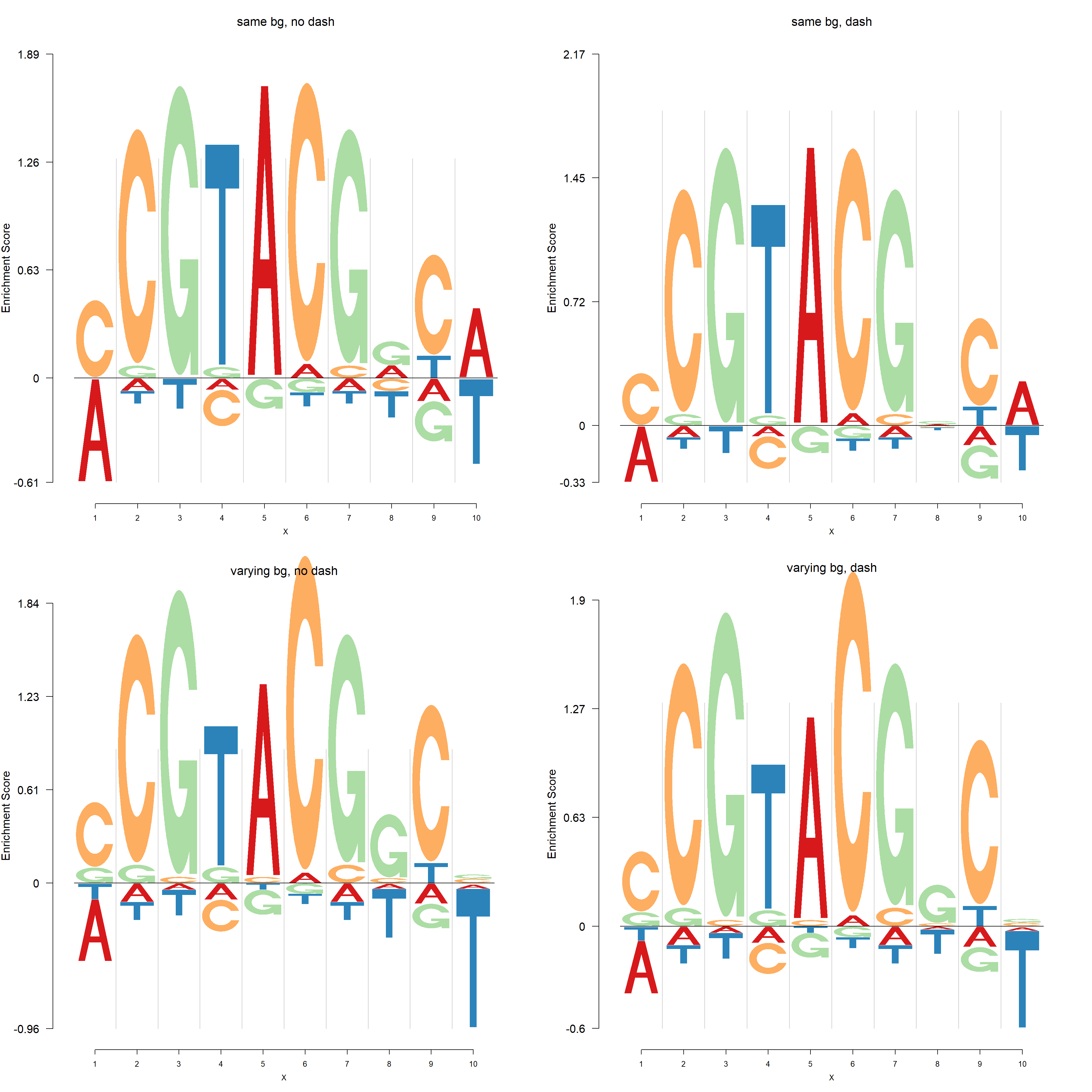
Session information
sessionInfo()R version 3.4.0 (2017-04-21)
Platform: x86_64-w64-mingw32/x64 (64-bit)
Running under: Windows 10 x64 (build 15063)
Matrix products: default
locale:
[1] LC_COLLATE=English_United States.1252
[2] LC_CTYPE=English_United States.1252
[3] LC_MONETARY=English_United States.1252
[4] LC_NUMERIC=C
[5] LC_TIME=English_United States.1252
attached base packages:
[1] grid stats graphics grDevices utils datasets methods
[8] base
other attached packages:
[1] dash_0.99.0 SQUAREM_2016.8-2 Logolas_1.1.2
loaded via a namespace (and not attached):
[1] Rcpp_0.12.12 digest_0.6.12 rprojroot_1.2
[4] backports_1.0.5 git2r_0.18.0 magrittr_1.5
[7] evaluate_0.10 stringi_1.1.5 LaplacesDemon_16.0.1
[10] rmarkdown_1.6 RColorBrewer_1.1-2 tools_3.4.0
[13] stringr_1.2.0 parallel_3.4.0 yaml_2.1.14
[16] compiler_3.4.0 htmltools_0.3.5 knitr_1.15.1 This R Markdown site was created with workflowr