Extended features of Logolas
Dongyue Xie
2017-08-23
Last updated: 2017-08-25
Code version: c6a9a06
Extended features of Logolas
Protein logo plot
User could use Logolas for protein sequence motif plot as well, as its logo library includes all the English alphabets and the 20 amino acids have a 1-letter representation using English alphabets.
Note that all one needs to do to build the logo plots is to specify the row names and column names as per the the logos and the stack labels and then fix the colors for the logos.
The default background probability is uniform and user could specify the background probability for each amino acid. One common used is from the BLOSUM62.
library(Logolas)
library(grid)
counts_mat <- rbind(c(0, 0, 100, 1, 2), c(4, 3, 30, 35, 2),
c(100, 0, 10, 2, 7),rep(0,5),
c(4, 2, 3, 7, 70), c(1, 8, 0, 60, 3),
rep(0, 5), c(4, 2, 100, 1, 1),
c(12, 8, 16, 7, 20), c(55, 0, 1, 0, 12),
rep(0,5), c(rep(0,3), 20, 0),
rep(0,5), c(0, 0, 30, 0, 22),
c(1, 0, 12, 3, 10), rep(0,5),
c(0, 1, 0, 34, 1), c(0, 1, 12, 35, 1),
c(0, 30, 1, 10, 2), c(0, 1, 4, 100, 2))

rownames(counts_mat) <- c("A", "R", "N", "D","C", "E", "Q", "G",
"H", "I", "L", "K", "M", "F", "P", "S",
"T", "W", "Y", "V")
colnames(counts_mat) <- c("Pos 1", "Pos 2", "Pos 3", "Pos 4", "Pos 5")
cols1 <- c(rev(RColorBrewer::brewer.pal(12, "Paired"))[c(3,4,7,8,11,12,5,6,9,10)],
RColorBrewer::brewer.pal(12, "Set3")[c(1,2,5,8,9)],
RColorBrewer::brewer.pal(9, "Set1")[c(9,7)],
RColorBrewer::brewer.pal(8, "Dark2")[c(3,4,8)])
color_profile <- list("type" = "per_row",
"col" = cols1)

grid.newpage()
layout.rows <- 1
layout.cols <- 2
top.vp <- viewport(layout=grid.layout(layout.rows,layout.cols, widths=unit(rep(2,layout.cols), rep("null",layout.cols)),heights=unit(rep(2,1), rep("null",1))))

plot_reg <- vpList()
l <- 1
for(i in 1:layout.rows){
  for(j in 1:layout.cols){
    plot_reg[[l]] <- viewport(layout.pos.col = j, layout.pos.row = i, name = paste0("plotlogo", l))
    l <- l+1
  }
}


plot_tree <- vpTree(top.vp, plot_reg)

pushViewport(plot_tree)
seekViewport(paste0("plotlogo", 1))

logomaker(counts_mat,
color_profile = color_profile,
newpage = FALSE,
frame_width = 1)

seekViewport(paste0("plotlogo", 2))

logomaker(counts_mat,
color_profile = color_profile,
bg=c(0.074,0.052,0.045,0.054,0.025,0.034,0.054,0.074,0.026,0.068,0.099,0.058,0.025,0.047,0.039,0.057,0.051,0.013,0.034,0.073),
newpage = FALSE,
pop_name = 'Logo plot with Varying background prob',
frame_width = 1)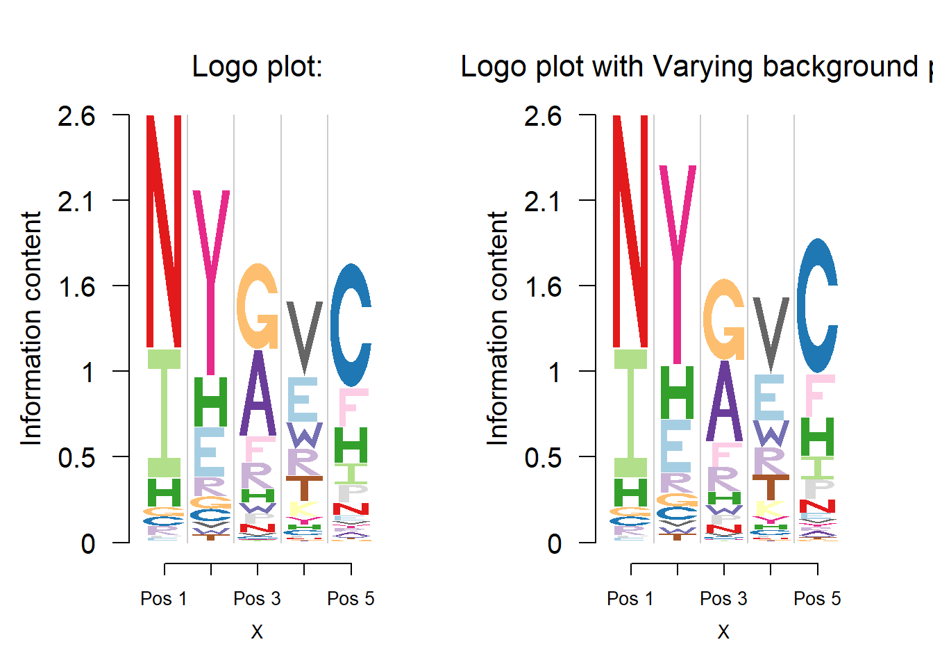
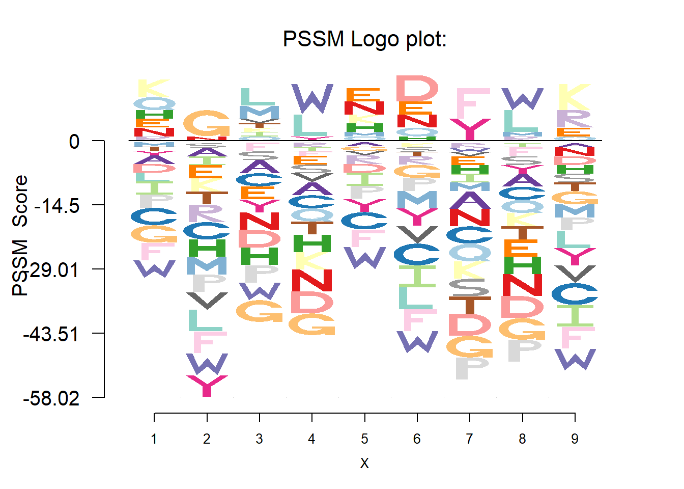
PSSM plot
Position-specific scoring matrix(PSSM) is constructed from a multiple alignment of a set of sequences. If a residue at a particular position is highly conserved(high relative frequency), it is given a high positive socre and the other residues are given high negative score. All residues are given scores near zero if the residues are all weakly conserved at that position.
The function logo_pssm plots the sequence logo based on the PSSM.
pssm 1 2 3 4 5 6 7 8 9
A -2 -2 -3 -3 -1 0 -4 -3 -1
R 1 -4 0 -1 -2 -2 -1 1 4
N 2 1 -4 -5 3 3 -4 -5 -2
D -2 0 -4 -5 -2 6 -5 -5 -2
C -4 -4 -3 -3 -4 -5 -4 -3 -5
Q 3 0 1 -3 1 2 -4 -3 1
E 2 -3 -3 -2 3 3 -2 -4 2
G -4 6 -5 -5 -1 -3 -5 -5 -3
H 2 -4 -4 -4 2 1 -2 -4 -2
I -3 -2 1 -1 -3 -5 -2 -1 -5
L -2 -5 4 5 0 -5 0 5 -4
K 4 -3 1 -4 2 -1 -4 -3 6
M -1 -4 3 0 1 -4 -2 1 -3
F -4 -5 -2 -1 -4 -5 7 -2 -5
P -3 -4 -4 0 -3 -3 -5 -5 -3
S 0 -1 -2 -2 0 -1 -4 -2 -2
T -1 -3 1 -3 0 -1 -4 -3 -2
W -4 -5 -4 7 -5 -5 -1 5 -5
Y -1 -5 -3 1 -3 -4 5 -2 -4
V 0 -4 1 -2 -1 -4 -1 0 -4logo_pssm(pssm,
color_profile = color_profile,
frame_width = 1
)
Mutation signature plot
Logolas could plot strings as logos. The first example is the cancer mutation signature. Detection of cancer mutaiton signatures is important in the study of the causes and mechanism of cancers. Usually we consider 6 possible mutation patterns(C to A/G/T, T to A/C/G). Suppose for a set of cell lines, we are provided data on the number of mutations (nucleotide substitions) and nucleotides at the flanking bases of the nucleotide substitution.
Shiraishi et al.(2015) proposed a parsimonious approach to model the mutation signatures, by assuming independence across mutation patterns. We apply it here on a demo example.
we use the symbols \(X>Y\) to denote the \(X\rightarrow Y\) substitutions. The data contains proportion of logos in each position : −2 left flanking, −1 left flanking, mutation, 1 right flanking and 2 right flanking. Note that \(X>Y\) type symbols occur only in the middle stack (column) as that is the mutation stack, while the nucleotides A, C, T and G occur only in the left two and right two flanking bases stacks (columns).
User may want to have the C in \(C>T\) to be of the same color as the C at the flankings and Logolas coloring profile provides the user the flexibility to color each symbol instead of a string. We use the color type per_symbol instead of the per_row profile we have been using so far. We consider a list of all symbols total_chars which is set as default to the list chosen above (so you can skip the total_chars argument below). However, if the user adds a symbol to the library (the process of doing that we show in the end), then the library is expected to grow and the user then might want to update the total_chars list by adding new symbols.
Another coloring option is per_column, in which we have a specific color for a specific column. This sort of coloring might be useful when the user wants to highlight the difference between columns. We provide an example of this next.
mFile <- system.file("Exfiles/pwm1", package="seqLogo")
m <- read.table(mFile)
p <- seqLogo::makePWM(m)
pwm_mat <- slot(p,name = "pwm")
mat1 <- cbind(pwm_mat[,c(3,4)], rep(0,4), pwm_mat[,c(5,6)]);
colnames(mat1) <- c("-2", "-1", "0", "1", "2")
mat2 <- cbind(rep(0,6), rep(0,6),
c(0.5, 0.2, 0.2, 0.05, 0.05, 0),
rep(0,6), rep(0,6))
rownames(mat2) <- c("C>T", "C>A", "C>G",
"T>A", "T>C", "T>G")
table <- rbind(mat1, mat2)

library(grid)
grid.newpage()
layout.rows <- 1
layout.cols <- 2
top.vp <- viewport(layout=grid.layout(layout.rows, layout.cols,
                                      widths=unit(rep(6,layout.cols), rep("null", 2)),
                                      heights=unit(c(20,50), rep("lines", 2))))

plot_reg <- vpList()
l <- 1
for(i in 1:layout.rows){
  for(j in 1:layout.cols){
    plot_reg[[l]] <- viewport(layout.pos.col = j, layout.pos.row = i, name = paste0("plotlogo", l))
    l <- l+1
  }
}


plot_tree <- vpTree(top.vp, plot_reg)

pushViewport(plot_tree)
seekViewport(paste0("plotlogo", 1))
color_profile <- list("type" = "per_row",
"col" = RColorBrewer::brewer.pal(dim(table)[1],name ="Spectral"))
logomaker(table,
          color_profile = color_profile,
          frame_width = 1,
          newpage = FALSE,
          xlab = "Position",
          ylab = "Information content")


seekViewport(paste0("plotlogo", 2))
cols = RColorBrewer::brewer.pal.info[RColorBrewer::brewer.pal.info$category == 'qual',]
col_vector = unlist(mapply(RColorBrewer::brewer.pal, cols$maxcolors, rownames(cols)))

total_chars = c("A", "B", "C", "D", "E", "F", "G", "H", "I", "J", "K", "L", "M", "N", "O",
"P", "Q", "R", "S", "T", "U", "V", "W", "X", "Y", "Z", "zero", "one", "two",
"three", "four", "five", "six", "seven", "eight", "nine", "dot", "comma",
"dash", "colon", "semicolon", "leftarrow", "rightarrow")

set.seed(20)
color_profile <- list("type" = "per_symbol",
"col" = sample(col_vector, length(total_chars), replace=FALSE))

logomaker(table,
          color_profile = color_profile,
          total_chars = total_chars,
          frame_width = 1,
          newpage = FALSE,
          xlab = "Position",
          ylab = "Information content")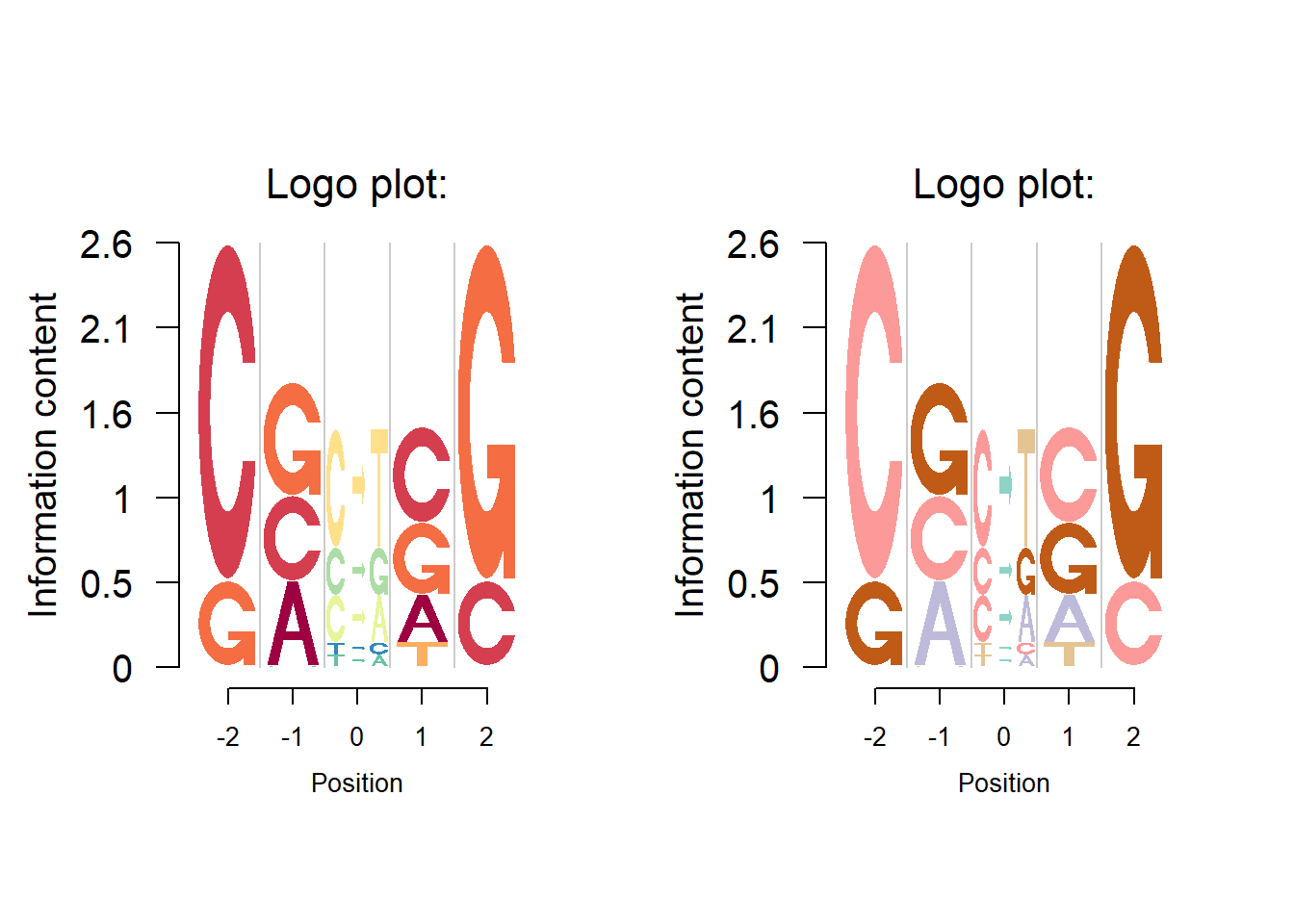
Full string plots
Logolas provides a handy visualization of strings, apart from the simple alphabet. We present two examples below.
Histone marks
In studies related to histone marks, one might be interested to see if certain histone marks are prominent than others in some cell lines or tissues or in some genomic regions. In this case, we apply Logolas on an example data from Koch et al (2007). The authors recorded number of histone modification sites identified by their algorithm which overlap with an intergenic sequence, intron, exon, gene start and gene end for the lymphoblastoid cell line, GM06990, in the ChIP-CHIP data. Note here that the histone mark symbols are alphanumeric, for example H3K4ME1.
mat <- rbind(c(326, 296, 81, 245, 71),
c(258, 228, 55, 273, 90),
c(145, 121, 29, 253, 85),
c(60, 52, 23, 180, 53),
c(150, 191, 63, 178, 63))
rownames(mat) <- c("H3K4ME1", "H3K4ME2", "H3K4ME3", "H3AC", "H4AC")
colnames(mat) <- c("Intergenic","Intron","Exon \n 1000 KB window",
"Gene start \n 1000 KB window","Gene end \n 1000 KB window")

color_profile <- list("type" = "per_row",
"col" = RColorBrewer::brewer.pal(dim(mat)[1],name ="Spectral"))

logomaker(mat,color_profile = color_profile,frame_width = 1)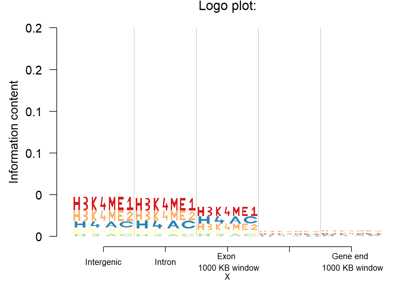
From the plot, it’s practical to see how the patterns of histone modification sites changes across genomic region types for that cell line.
Document mining
Further, the logos could include the punctuation marks as well like the full stop.
Here we build a logo plot of the field categories of manuscipts submitted on aRxiv by 4 professors from Department of Statistics, University of Chicago. Note that the field categories here are a combination of numbers, alphabets, dots and dashes.
library(aRxiv)
rec1 <- aRxiv::arxiv_search('au:"Matthew Stephens"', limit=50)
rec2 <- aRxiv::arxiv_search('au:"John Lafferty"', limit=50)
rec3 <- aRxiv::arxiv_search('au:"Wei Biao Wu"', limit=50)
rec4 <- aRxiv::arxiv_search('au:"Peter Mccullagh"', limit=50)

primary_categories_1 <- toupper(rec1$primary_category)
primary_categories_2 <- toupper(rec2$primary_category)
primary_categories_3 <- toupper(rec3$primary_category)
primary_categories_4 <- toupper(rec4$primary_category)

factor_levels <- unique(c(unique(primary_categories_1),
unique(primary_categories_2),
unique(primary_categories_3),
unique(primary_categories_4)))

primary_categories_1 <- factor(primary_categories_1, levels=factor_levels)
primary_categories_2 <- factor(primary_categories_2, levels=factor_levels)
primary_categories_3 <- factor(primary_categories_3, levels=factor_levels)
primary_categories_4 <- factor(primary_categories_4, levels=factor_levels)

tab_data <- cbind(table(primary_categories_1),
table(primary_categories_2),
table(primary_categories_3),
table(primary_categories_4))

colnames(tab_data) <- c("Matthew Stephens",
"John Lafferty",
"Wei Biao Wu",
"Peter McCullagh")
tab_data <- as.matrix(tab_data)

color_profile <- list("type" = "per_row",
"col" = RColorBrewer::brewer.pal(dim(tab_data)[1],
name = "Spectral"))

logomaker(tab_data,
        color_profile = color_profile,
        frame_width = 1,
        pop_name = "arXiv field categories of UChicago STAT professors",
        xlab = "Professors",
        ylab = "Information content")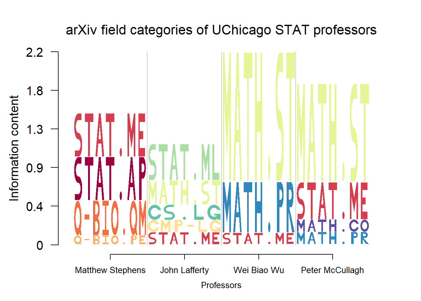
Combining plots with R graphs
User could combine logo plots from Logolas with plots from the other R graphs such as R base graphics and ggplot2 graph.
library(ggplot2)
library(grid)
library(gridBase)

m = matrix(rep(0,48),4,12)
m[1,] = c(0,0,2.5,7,0,0,0,0,0,0,1,2)
m[2,] = c(4,6,3,1,0,0,0,0,0,5,0,2)
m[3,] = c(0,0,0,0,0,1,8,0,0,1,1,2)
m[4,] = c(4,2,2.5,0,8,7,0,8,8,2,6,2)
rownames(m) = c("A", "C", "G", "T")
colnames(m) = 1:12
m=m/8

color_profile = list("type" = "per_row",
                     "col" = RColorBrewer::brewer.pal(4,name ="Spectral"))

mtcars$gear <- factor(mtcars$gear,levels=c(3,4,5),
                      labels=c("3gears","4gears","5gears"))
mtcars$am <- factor(mtcars$am,levels=c(0,1),
                    labels=c("Automatic","Manual"))
mtcars$cyl <- factor(mtcars$cyl,levels=c(4,6,8),
                     labels=c("4cyl","6cyl","8cyl"))


grid.newpage()
layout.rows <- 2
layout.cols <- 2
top.vp <- viewport(layout=grid.layout(layout.rows, layout.cols,
                                      widths=unit(rep(2,layout.cols), rep("null", layout.cols)),
                                      heights=unit(rep(2,1), rep("null",1))))

plot_reg <- vpList()
l <- 1
for(i in 1:layout.rows){
  for(j in 1:layout.cols){
    plot_reg[[l]] <- viewport(layout.pos.col = j, layout.pos.row = i, name = paste0("plotlogo", l))
    l <- l+1
  }
}


plot_tree <- vpTree(top.vp, plot_reg)

pushViewport(plot_tree)
seekViewport(paste0("plotlogo", 1))
logomaker(m,xlab = 'position',color_profile = color_profile,
          bg = c(0.28, 0.22, 0.24, 0.26),
          frame_width = 1,
          newpage = FALSE,
          control = list(viewport.margin.left = 5))


seekViewport(paste0("plotlogo", 2))
vp3 = viewport(width=0.8, height=0.8, x = 0.5, y = 0.5)
p <- qplot(mpg, data=mtcars, geom="density")
print(p, vp = vp3)

seekViewport(paste0("plotlogo", 3))
vp3 = viewport(height = 1, width = 1)
pushViewport(vp3)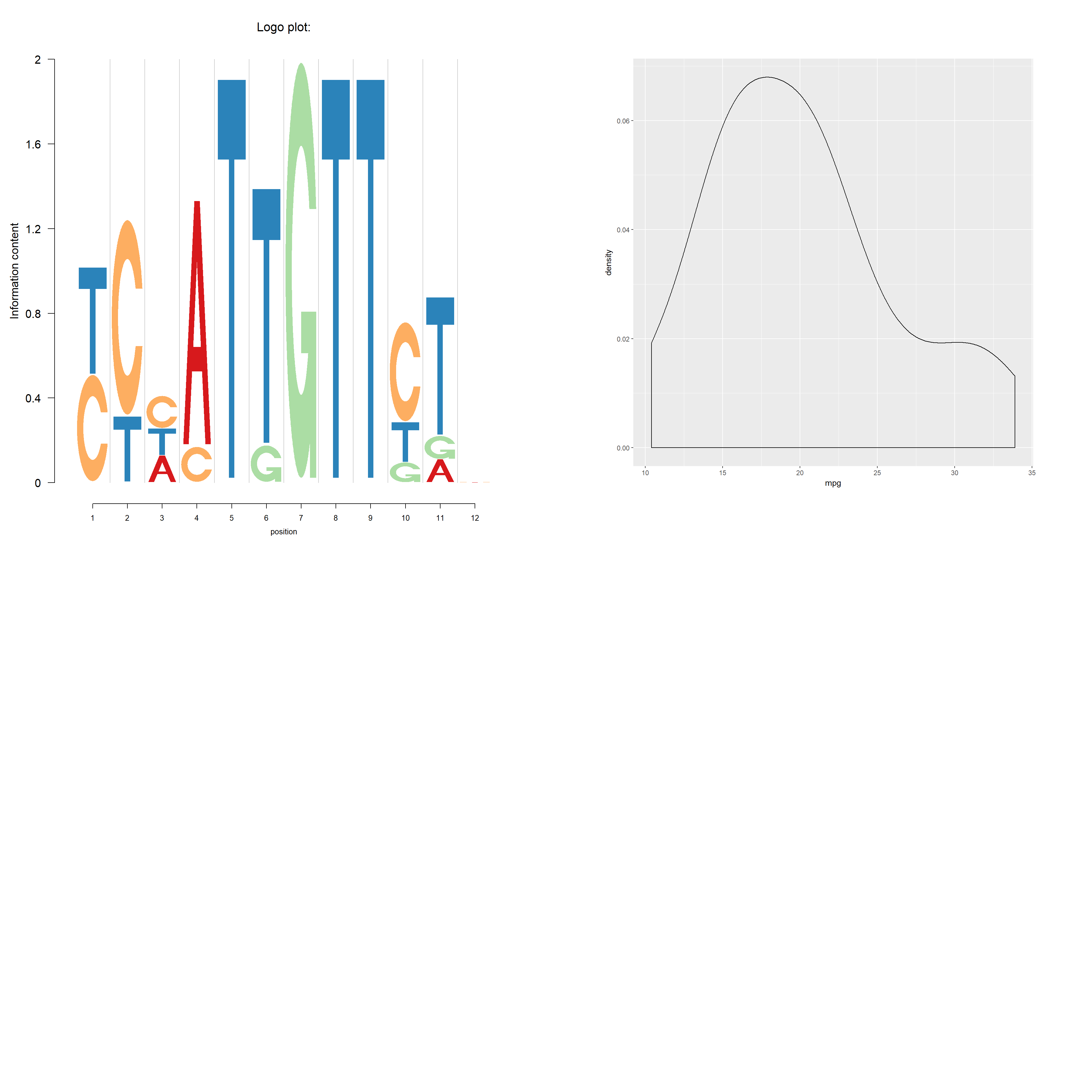
par(fig=gridFIG())
par(gridPAR())
par(new=TRUE)
par(mar = c(3, 3, 1, 1))
plot(1:10, type="b")
Session information
sessionInfo()R version 3.4.0 (2017-04-21)
Platform: x86_64-w64-mingw32/x64 (64-bit)
Running under: Windows 10 x64 (build 15063)
Matrix products: default
locale:
[1] LC_COLLATE=English_United States.1252
[2] LC_CTYPE=English_United States.1252
[3] LC_MONETARY=English_United States.1252
[4] LC_NUMERIC=C
[5] LC_TIME=English_United States.1252
attached base packages:
[1] grid stats graphics grDevices utils datasets methods
[8] base
other attached packages:
[1] gridBase_0.4-7 ggplot2_2.2.1 aRxiv_0.5.16 dash_0.99.0
[5] SQUAREM_2016.8-2 Logolas_1.1.2
loaded via a namespace (and not attached):
[1] Rcpp_0.12.12 compiler_3.4.0 RColorBrewer_1.1-2
[4] git2r_0.18.0 plyr_1.8.4 tools_3.4.0
[7] digest_0.6.12 evaluate_0.10 tibble_1.3.3
[10] gtable_0.2.0 rlang_0.1.1 curl_2.5
[13] yaml_2.1.14 seqLogo_1.42.0 httr_1.2.1
[16] stringr_1.2.0 knitr_1.15.1 stats4_3.4.0
[19] rprojroot_1.2 R6_2.2.0 XML_3.98-1.6
[22] rmarkdown_1.6 magrittr_1.5 backports_1.0.5
[25] scales_0.4.1 htmltools_0.3.5 colorspace_1.3-2
[28] labeling_0.3 stringi_1.1.5 lazyeval_0.2.0
[31] munsell_0.4.3 This R Markdown site was created with workflowr