Last updated: 2018-05-09

workflowr checks: (Click a bullet for more information)

✔ R Markdown file: up-to-date

Great! Since the R Markdown file has been committed to the Git repository, you know the exact version of the code that produced these results.
✔ Environment: empty

Great job! The global environment was empty. Objects defined in the global environment can affect the analysis in your R Markdown file in unknown ways. For reproduciblity it’s best to always run the code in an empty environment.
✔ Seed: set.seed(20180501)

The command set.seed(20180501) was run prior to running the code in the R Markdown file. Setting a seed ensures that any results that rely on randomness, e.g. subsampling or permutations, are reproducible.
✔ Session information: recorded

Great job! Recording the operating system, R version, and package versions is critical for reproducibility.
✔ Repository version: 714d35a
Great! You are using Git for version control. Tracking code development and connecting the code version to the results is critical for reproducibility. The version displayed above was the version of the Git repository at the time these results were generated.

Note that you need to be careful to ensure that all relevant files for the analysis have been committed to Git prior to generating the results (you can use wflow_publish or wflow_git_commit). workflowr only checks the R Markdown file, but you know if there are other scripts or data files that it depends on. Below is the status of the Git repository when the results were generated:
```
Ignored files:
    Ignored:    .Rhistory
    Ignored:    .Rproj.user/
    Ignored:    log/

Untracked files:
    Untracked:  analysis/overdis.Rmd
    Untracked:  docs/figure/ashpmean.Rmd/

Unstaged changes:
    Modified:   analysis/nugget.Rmd
```
Note that any generated files, e.g. HTML, png, CSS, etc., are not included in this status report because it is ok for generated content to have uncommitted changes.

Expand here to see past versions:

File	Version	Author	Date	Message
Rmd	714d35a	Dongyue	2018-05-09	one iteration ash poisson
Rmd	4a16b9f	Dongyue	2018-05-09	one iteration ash poisson

library(smashr)
library(ashr)

Warning: package 'ashr' was built under R version 3.4.4

#' smash generaliation function, expansion around ash posterior mean


#' @param x: a vector of observations
#' @param sigma: standard deviations, scalar.
#' @param family: choice of wavelet basis to be used, as in wavethresh.
#' @param niter: number of iterations for IRLS
#' @param tol: tolerance of the criterion to stop the iterations
#' @param ashp: whether expand around ash posterior mean 
#' @param robust: whether set the highest resolution wavelet coeffs to 0
#' @param verbose: whether print out the number of iterations to converge.

smash.gen=function(x,sigma,family='DaubExPhase',
                   ashp=TRUE,verbose=FALSE, robust=FALSE,
                   niter=30,tol=1e-2){
  mu=c()
  s=c()
  y=c()
  munorm=c()
  #apply ash to poisson data?
  if(ashp){
    pmean=ash(rep(0,length(x)),1,lik=lik_pois(x))$result$PosteriorMean
    mu=rbind(mu,pmean)
    s=rbind(s,1/mu)
    y0=log(mu)+(x-mu)/mu
  }else{
    mu=rbind(mu,rep(mean(x),length(x)))
    s=rbind(s,1/mu)
    y0=log(mean(x))+(x-mean(x))/mean(x)
  }
  #set wavelet coeffs to 0?
  if(robust){
    wds=wd(y0,family = family,filter.number = filter.number)
    wtd=threshold(wds, levels = wds$nlevels-1,  policy="manual",value = Inf) 
    y=rbind(y,wr(wtd))
  }else{
    y=rbind(y,y0)
  }
  for(i in 1:niter){
    vars=ifelse(s[i,]<0,1e-8,s[i,])
    mu.hat=smash.gaus(y[i,],sigma=sqrt(vars))#mu.hat is \mu_t+E(u_t|y)
    mu=rbind(mu,mu.hat)
    munorm[i]=norm(mu.hat-mu[i,],'2')
    if(munorm[i]<tol){
      if(verbose){
        message(sprintf('Converge after %i iterations',i))
      }
      break
    }
    #update m and s_t
    mt=exp(mu.hat)
    s=rbind(s,1/mt)
    y=rbind(y,log(mt)+(x-mt)/mt)
    
    
  }
  mu.hat=smash.gaus(y[i,],sigma = sqrt(sigma^2+ifelse(s[i,]<0,1e-8,s[i,])))
  return(list(mu.hat=mu.hat,mu=mu,s=s,y=y,munorm=munorm))
}

#' Simulation study comparing smash and smashgen

simu_study=function(m,sigma,seed=1234,
                    niter=1,family='DaubExPhase',ashp=TRUE,verbose=FALSE,robust=FALSE,
                    tol=1e-2,reflect=FALSE){
  set.seed(seed)
  lamda=exp(m+rnorm(length(m),0,sigma))
  x=rpois(length(m),lamda)
  #fit data
  smash.out=smash.poiss(x,reflect=reflect)
  smash.gen.out=smash.gen(x,sigma=sigma,niter=niter,family = family,tol=tol,ashp=ashp,verbose=verbose)
  return(list(smash.out=smash.out,smash.gen.out=exp(smash.gen.out$mu.hat),smash.gen.est=smash.gen.out,x=x,loglik=smash.gen.out$loglik))
}

Simulation 1: Constant trend Poisson nugget

\(\sigma=0.01\)

library(smashr)
m=rep(3,256)
simu.out=simu_study(m,0.01)
simu.out.conv=simu_study(m,0.01,niter = 30)
#par(mfrow = c(1,2))

plot(simu.out$x,col = "gray80" ,ylab = '')
lines(simu.out.conv$smash.gen.out, col = "blue", lwd = 2)
lines(simu.out$smash.gen.out, col = "red", lwd = 2)

lines(exp(m))
legend("topright", # places a legend at the appropriate place
       c("truth","smash-gen-1iter","converged"), # puts text in the legend
       lty=c(1,1,1), # gives the legend appropriate symbols (lines)
       lwd=c(1,1,1),
       cex = 1,
       col=c("black","red", "blue"))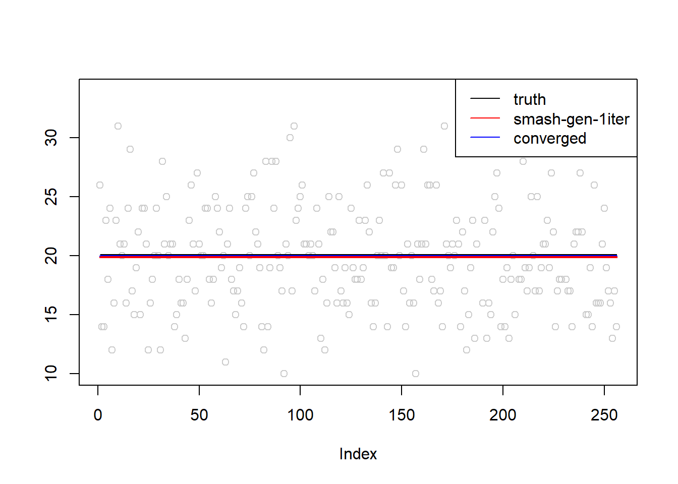

\(\sigma=0.1\)

simu.out=simu_study(m,0.1)
simu.out.conv=simu_study(m,0.1,niter=30)
#par(mfrow = c(1,2))

plot(simu.out$x,col = "gray80" ,ylab = '')
lines(simu.out$smash.gen.out, col = "red", lwd = 2)
lines(simu.out.conv$smash.gen.out, col = "blue", lwd = 2)
lines(exp(m))
legend("topright", # places a legend at the appropriate place
       c("truth","smash-gen-1iter","converged"), # puts text in the legend
       lty=c(1,1,1), # gives the legend appropriate symbols (lines)
       lwd=c(1,1,1),
       cex = 1,
       col=c("black","red", "blue"))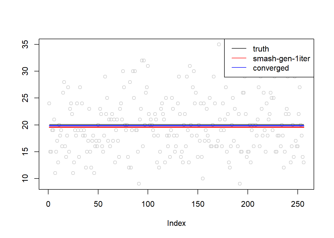

\(\sigma=0.5\)

simu.out=simu_study(m,0.5)
simu.out.conv=simu_study(m,0.5,niter=30)
#par(mfrow = c(1,2))

plot(simu.out$x,col = "gray80" ,ylab = '')
lines(simu.out.conv$smash.gen.out, col = "blue", lwd = 2)
lines(simu.out$smash.gen.out, col = "red", lwd = 2)

lines(exp(m))
legend("topright", # places a legend at the appropriate place
       c("truth","smash-gen-1iter","converged"), # puts text in the legend
       lty=c(1,1,1), # gives the legend appropriate symbols (lines)
       lwd=c(1,1,1),
       cex = 1,
       col=c("black","red", "blue"))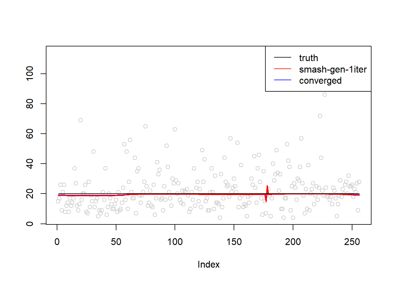

\(\sigma=1\)

simu.out=simu_study(m,1)
simu.out.conv=simu_study(m,1,niter=30)
#par(mfrow = c(1,2))

plot(simu.out$x,col = "gray80" ,ylab = '')
lines(simu.out.conv$smash.gen.out, col = "blue", lwd = 2)
lines(simu.out$smash.gen.out, col = "red", lwd = 2)

lines(exp(m))
legend("topright", # places a legend at the appropriate place
       c("truth","smash-gen-1iter","converged"), # puts text in the legend
       lty=c(1,1,1), # gives the legend appropriate symbols (lines)
       lwd=c(1,1,1),
       cex = 1,
       col=c("black","red", "blue"))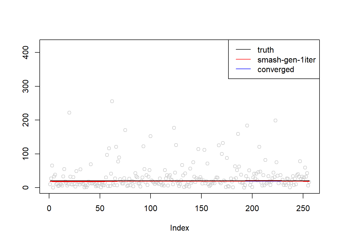

Simulation 2: Step trend

\(\sigma=0.01\)

m=c(rep(3,128), rep(5, 128), rep(6, 128), rep(3, 128))
simu.out=simu_study(m,0.01)
simu.out.conv=simu_study(m,0.01,niter=30)
#par(mfrow = c(1,2))

plot(simu.out$x,col = "gray80" ,ylab = '')
lines(simu.out.conv$smash.gen.out, col = "blue", lwd = 2)
lines(simu.out$smash.gen.out, col = "red", lwd = 2)
lines(exp(m))
legend("topleft", # places a legend at the appropriate place
       c("truth","smash-gen-1iter","converged"), # puts text in the legend
       lty=c(1,1,1), # gives the legend appropriate symbols (lines)
       lwd=c(1,1,1),
       cex = 1,
       col=c("black","red", "blue"))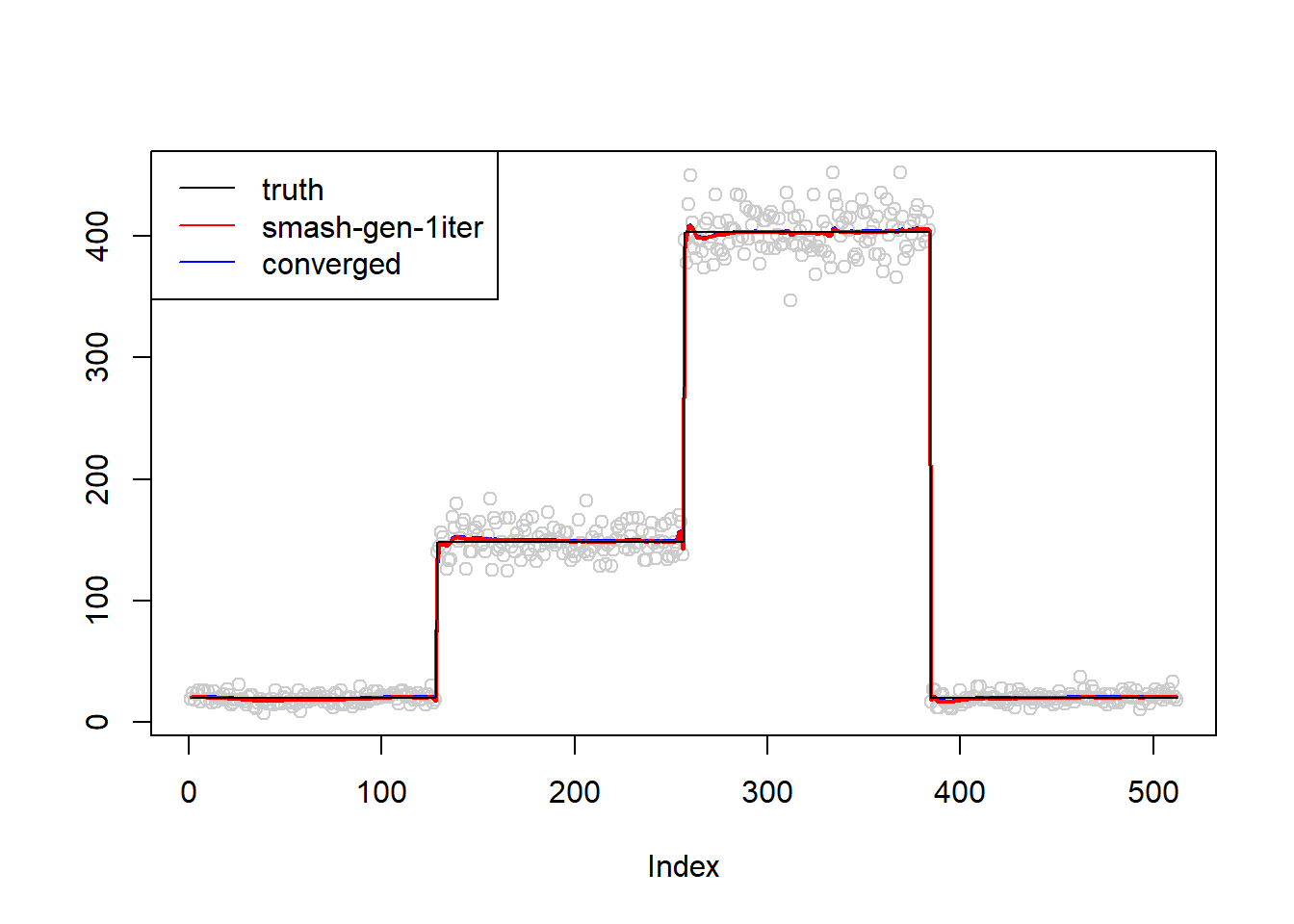

\(\sigma=0.1\)

simu.out=simu_study(m,0.1)
simu.out.conv=simu_study(m,0.1,niter=30)
#par(mfrow = c(1,2))

plot(simu.out$x,col = "gray80" ,ylab = '')
lines(simu.out.conv$smash.gen.out, col = "blue", lwd = 2)
lines(simu.out$smash.gen.out, col = "red", lwd = 2)
lines(exp(m))
legend("topleft", # places a legend at the appropriate place
       c("truth","smash-gen-1iter","converged"), # puts text in the legend
       lty=c(1,1,1), # gives the legend appropriate symbols (lines)
       lwd=c(1,1,1),
       cex = 1,
       col=c("black","red", "blue"))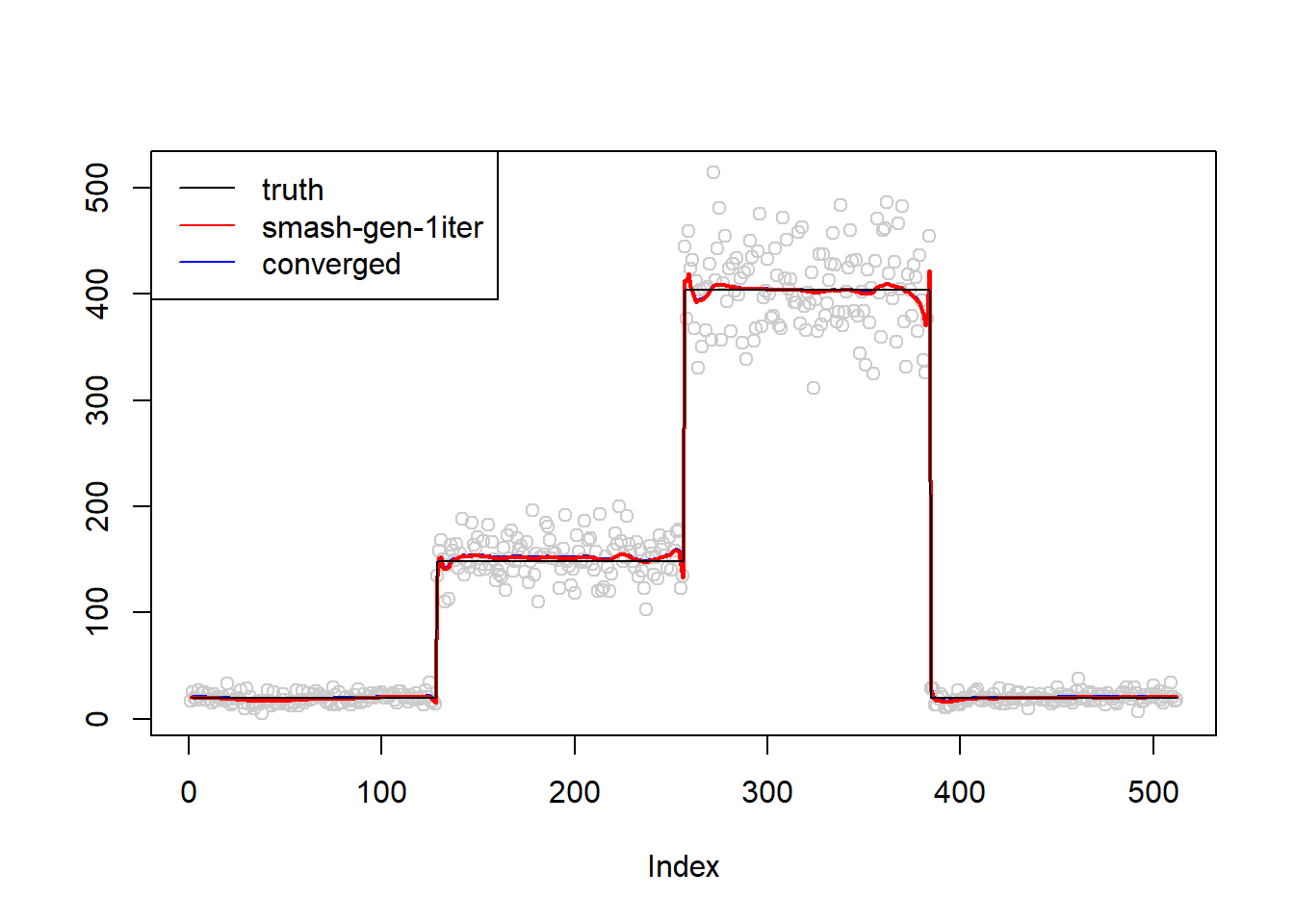

\(\sigma=0.5\)

simu.out=simu_study(m,0.5)
simu.out.conv=simu_study(m,0.5,niter=30)
#par(mfrow = c(1,2))

plot(simu.out$x,col = "gray80" ,ylab = '')
lines(simu.out.conv$smash.gen.out, col = "blue", lwd = 2)
lines(simu.out$smash.gen.out, col = "red", lwd = 2)
lines(exp(m))
legend("topleft", # places a legend at the appropriate place
       c("truth","smash-gen-1iter","converged"), # puts text in the legend
       lty=c(1,1,1), # gives the legend appropriate symbols (lines)
       lwd=c(1,1,1),
       cex = 1,
       col=c("black","red", "blue"))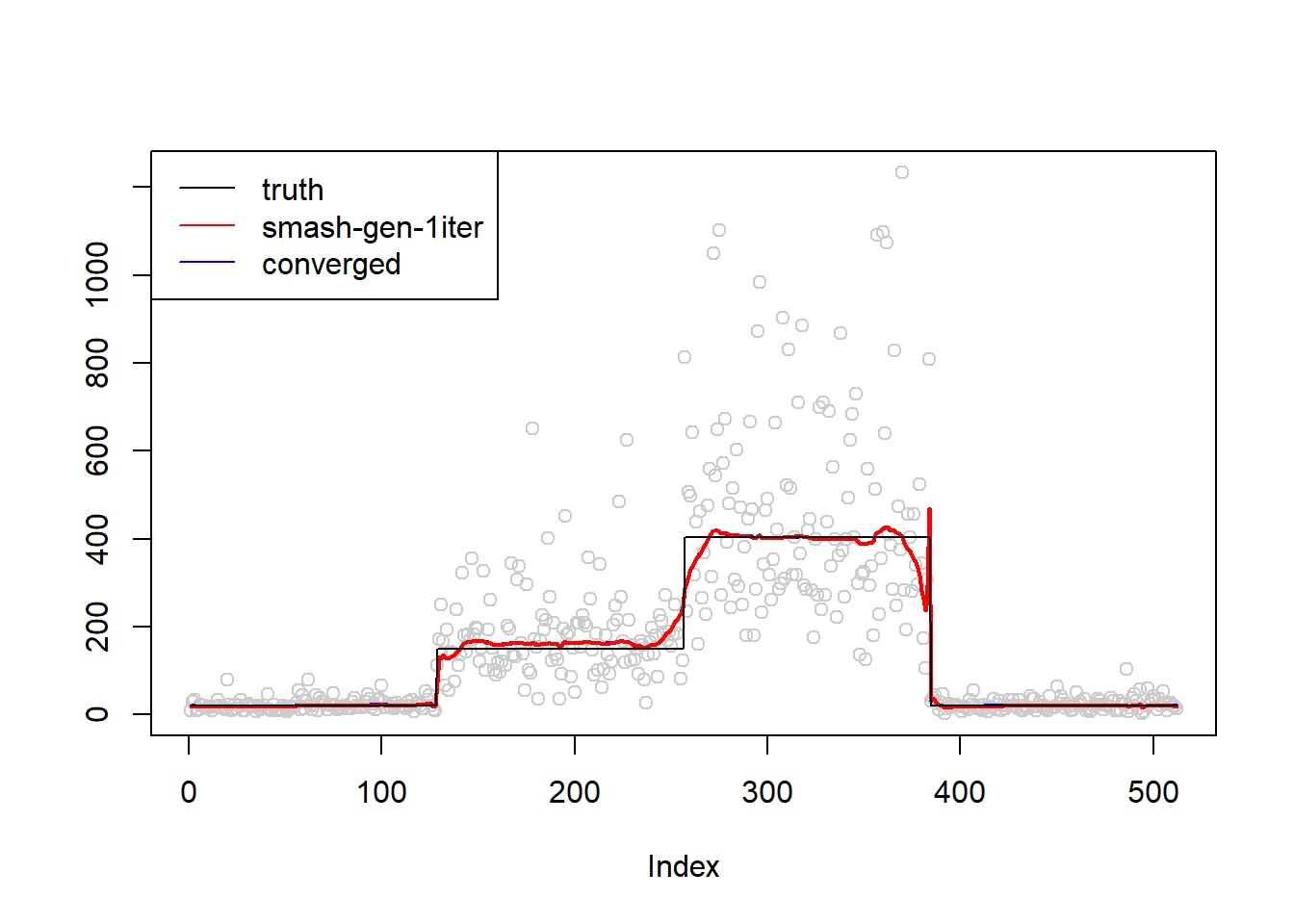

\(\sigma=1\)

simu.out=simu_study(m,1)
simu.out.conv=simu_study(m,1,niter=30)
#par(mfrow = c(1,2))

plot(simu.out$x,col = "gray80" ,ylab = '')
lines(simu.out.conv$smash.gen.out, col = "blue", lwd = 2)
lines(simu.out$smash.gen.out, col = "red", lwd = 2)
lines(exp(m))
legend("topleft", # places a legend at the appropriate place
       c("truth","smash-gen-1iter","converged"), # puts text in the legend
       lty=c(1,1,1), # gives the legend appropriate symbols (lines)
       lwd=c(1,1,1),
       cex = 1,
       col=c("black","red", "blue"))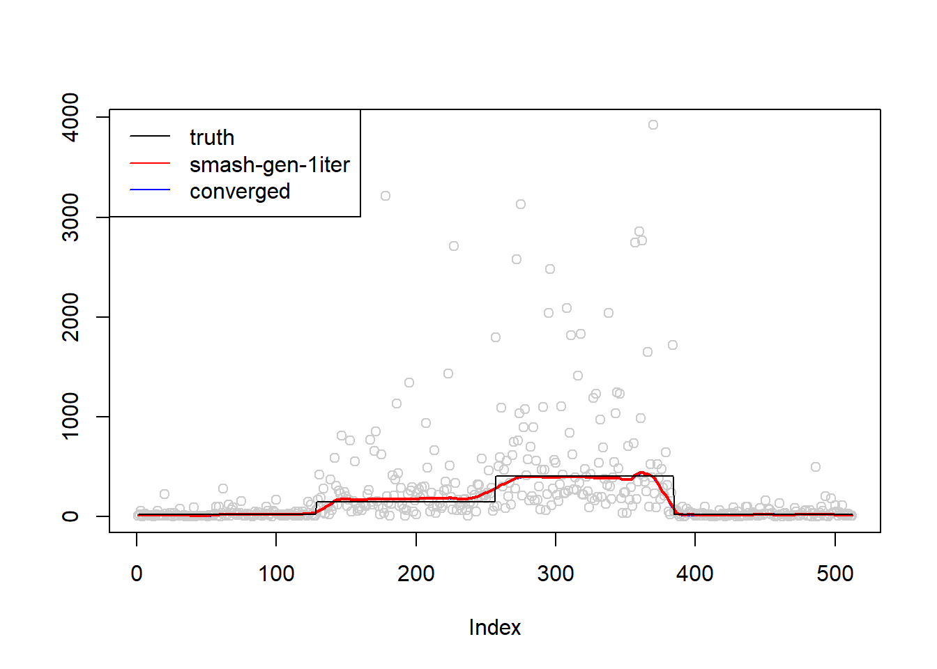

Simulation 3: Oscillating Poisson nugget

\(\sigma=0.01\)

m=c()
for(k in 1:8){
    m=c(m, rep(1,15), rep(5, 15))
}
m=c(m,rep(1,16))
simu.out=simu_study(m,0.01)
simu.out.conv=simu_study(m,0.01,niter=30)
#par(mfrow = c(1,2))

plot(simu.out$x,col = "gray80" ,ylab = '')
lines(simu.out.conv$smash.gen.out, col = "blue", lwd = 2)
lines(simu.out$smash.gen.out, col = "red", lwd = 2)
lines(exp(m))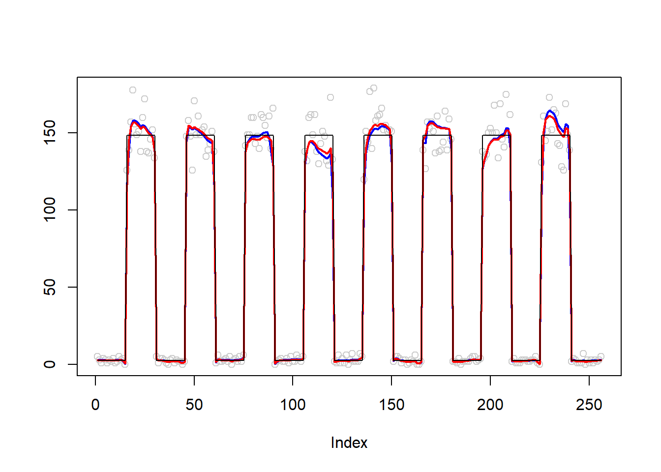

# legend("topleft", # places a legend at the appropriate place
#        c("truth","smash-gen-1iter","converged"), # puts text in the legend
#        lty=c(1,1,1), # gives the legend appropriate symbols (lines)
#        lwd=c(1,1,1),
#        cex = 1,
#        col=c("black","red", "blue"))

\(\sigma=0.1\)

simu.out=simu_study(m,0.1)
simu.out.conv=simu_study(m,0.1,niter=30)
#par(mfrow = c(1,2))

plot(simu.out$x,col = "gray80" ,ylab = '')
lines(simu.out.conv$smash.gen.out, col = "blue", lwd = 2)
lines(simu.out$smash.gen.out, col = "red", lwd = 2)
lines(exp(m))
legend("topleft", # places a legend at the appropriate place
       c("truth","smash-gen-1iter","converged"), # puts text in the legend
       lty=c(1,1,1), # gives the legend appropriate symbols (lines)
       lwd=c(1,1,1),
       cex = 1,
       col=c("black","red", "blue"))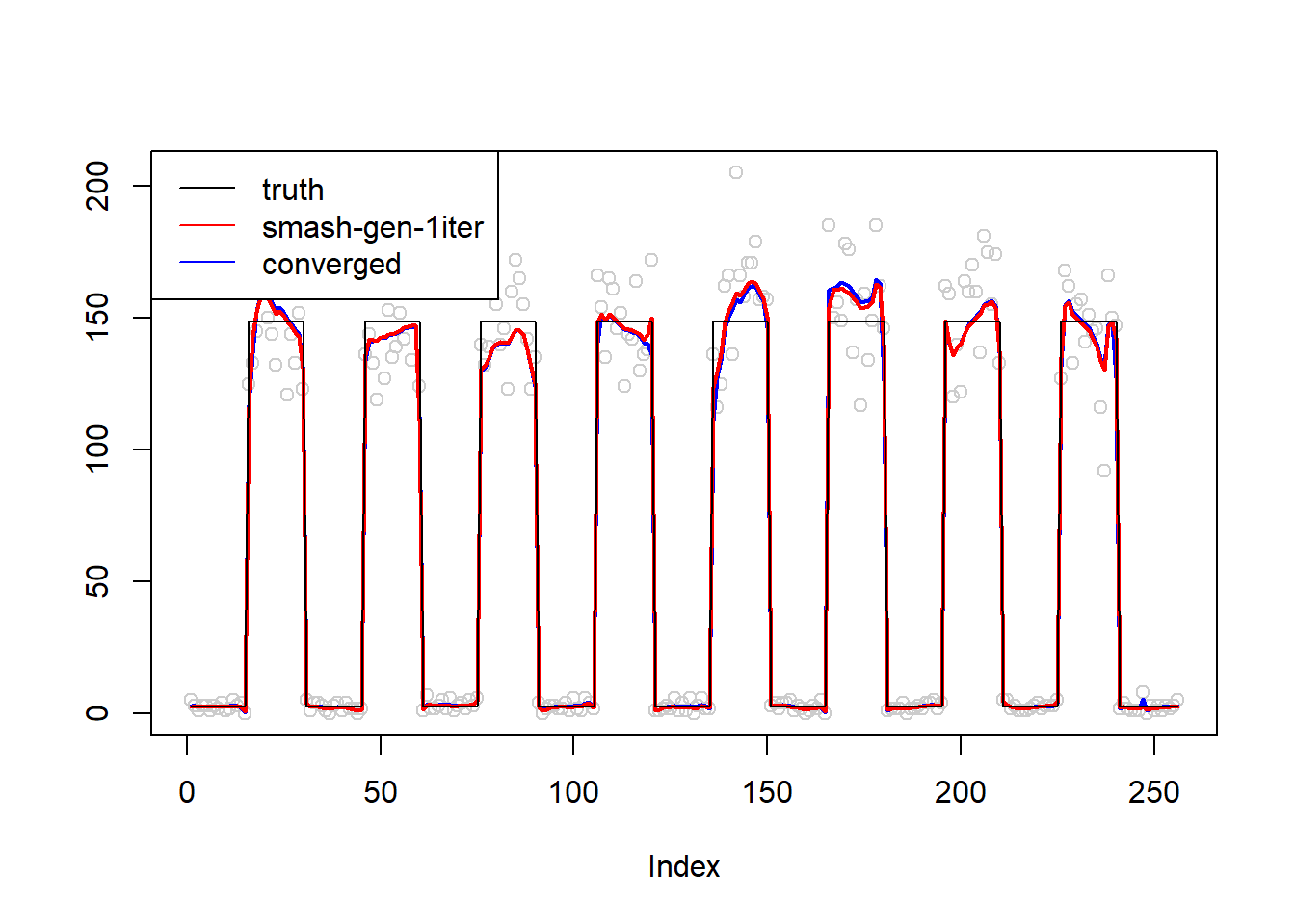

\(\sigma=0.5\)

simu.out=simu_study(m,0.5)
simu.out.conv=simu_study(m,0.5,niter=30)
#par(mfrow = c(1,2))

plot(simu.out$x,col = "gray80" ,ylab = '')
lines(simu.out.conv$smash.gen.out, col = "blue", lwd = 2)
lines(simu.out$smash.gen.out, col = "red", lwd = 2)
lines(exp(m))
legend("topleft", # places a legend at the appropriate place
       c("truth","smash-gen-1iter","converged"), # puts text in the legend
       lty=c(1,1,1), # gives the legend appropriate symbols (lines)
       lwd=c(1,1,1),
       cex = 1,
       col=c("black","red", "blue"))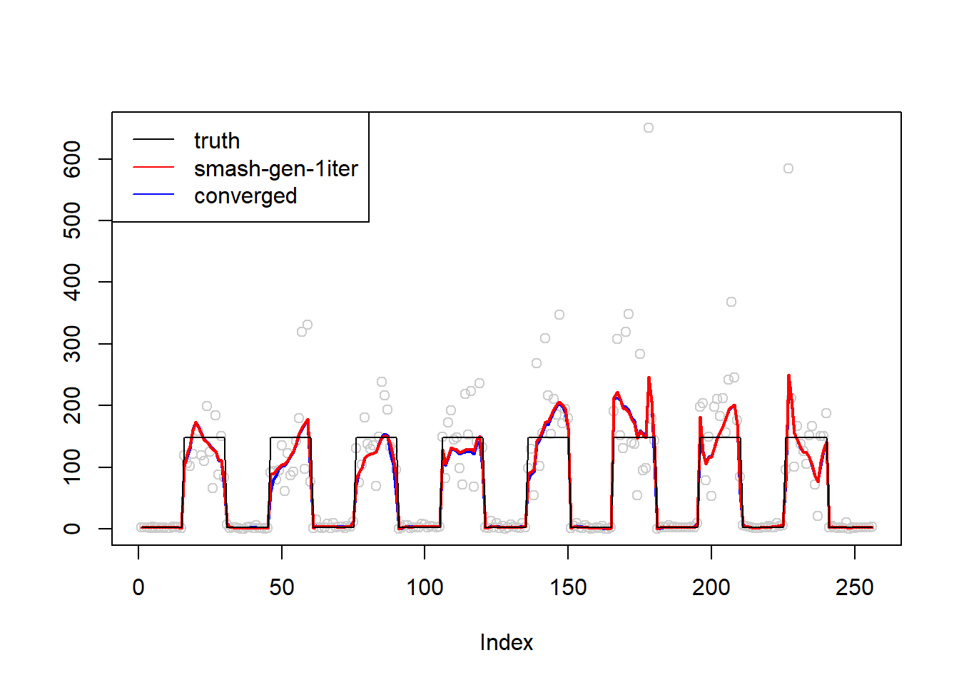

\(\sigma=1\)

simu.out=simu_study(m,1)

Warning in REBayes::KWDual(A, rep(1, k), normalize(w), control = control): estimated mixing distribution has some negative values:
               consider reducing rtol

Warning in mixIP(matrix_lik = structure(c(0, 0, 0, 0, 0, 0, 0, 0, 0,
0, : Optimization step yields mixture weights that are either too small,
or negative; weights have been corrected and renormalized after the
optimization.

Warning in REBayes::KWDual(A, rep(1, k), normalize(w), control = control): estimated mixing distribution has some negative values:
               consider reducing rtol

Warning in mixIP(matrix_lik = structure(c(0, 0, 0, 0, 0, 0, 0, 0, 0,
0, : Optimization step yields mixture weights that are either too small,
or negative; weights have been corrected and renormalized after the
optimization.

simu.out.conv=simu_study(m,1,niter=30)

Warning in REBayes::KWDual(A, rep(1, k), normalize(w), control = control): estimated mixing distribution has some negative values:
               consider reducing rtol

Warning in mixIP(matrix_lik = structure(c(0, 0, 0, 0, 0, 0, 0, 0, 0,
0, : Optimization step yields mixture weights that are either too small,
or negative; weights have been corrected and renormalized after the
optimization.

Warning in REBayes::KWDual(A, rep(1, k), normalize(w), control = control): estimated mixing distribution has some negative values:
               consider reducing rtol

Warning in mixIP(matrix_lik = structure(c(0, 0, 0, 0, 0, 0, 0, 0, 0,
0, : Optimization step yields mixture weights that are either too small,
or negative; weights have been corrected and renormalized after the
optimization.

#par(mfrow = c(1,2))

plot(simu.out$x,col = "gray80" ,ylab = '')
lines(simu.out.conv$smash.gen.out, col = "blue", lwd = 2)
lines(simu.out$smash.gen.out, col = "red", lwd = 2)
lines(exp(m))
legend("topleft", # places a legend at the appropriate place
       c("truth","smash-gen-1iter","converged"), # puts text in the legend
       lty=c(1,1,1), # gives the legend appropriate symbols (lines)
       lwd=c(1,1,1),
       cex = 1,
       col=c("black","red", "blue"))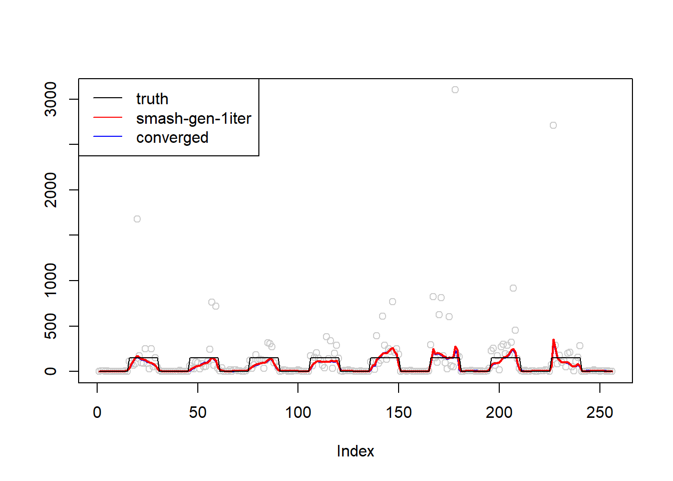

Simulation 4: Bumps

\(\sigma=0.01\)

m=seq(0,1,length.out = 256)
h = c(4, 5, 3, 4, 5, 4.2, 2.1, 4.3, 3.1, 5.1, 4.2)
w = c(0.005, 0.005, 0.006, 0.01, 0.01, 0.03, 0.01, 0.01, 0.005,0.008,0.005)
t=c(.1,.13,.15,.23,.25,.4,.44,.65,.76,.78,.81)
f = c()
for(i in 1:length(m)){
  f[i]=sum(h*(1+((m[i]-t)/w)^4)^(-1))
}
m=f
simu.out=simu_study(m,0.01)
simu.out.conv=simu_study(m,0.01,niter=30)
#par(mfrow = c(1,2))

plot(simu.out$x,col = "gray80" ,ylab = '')
lines(simu.out.conv$smash.gen.out, col = "blue", lwd = 2)
lines(simu.out$smash.gen.out, col = "red", lwd = 2)
lines(exp(m))
legend("topright", # places a legend at the appropriate place
       c("truth","smash-gen-1iter","converged"), # puts text in the legend
       lty=c(1,1,1), # gives the legend appropriate symbols (lines)
       lwd=c(1,1,1),
       cex = 1,
       col=c("black","red", "blue"))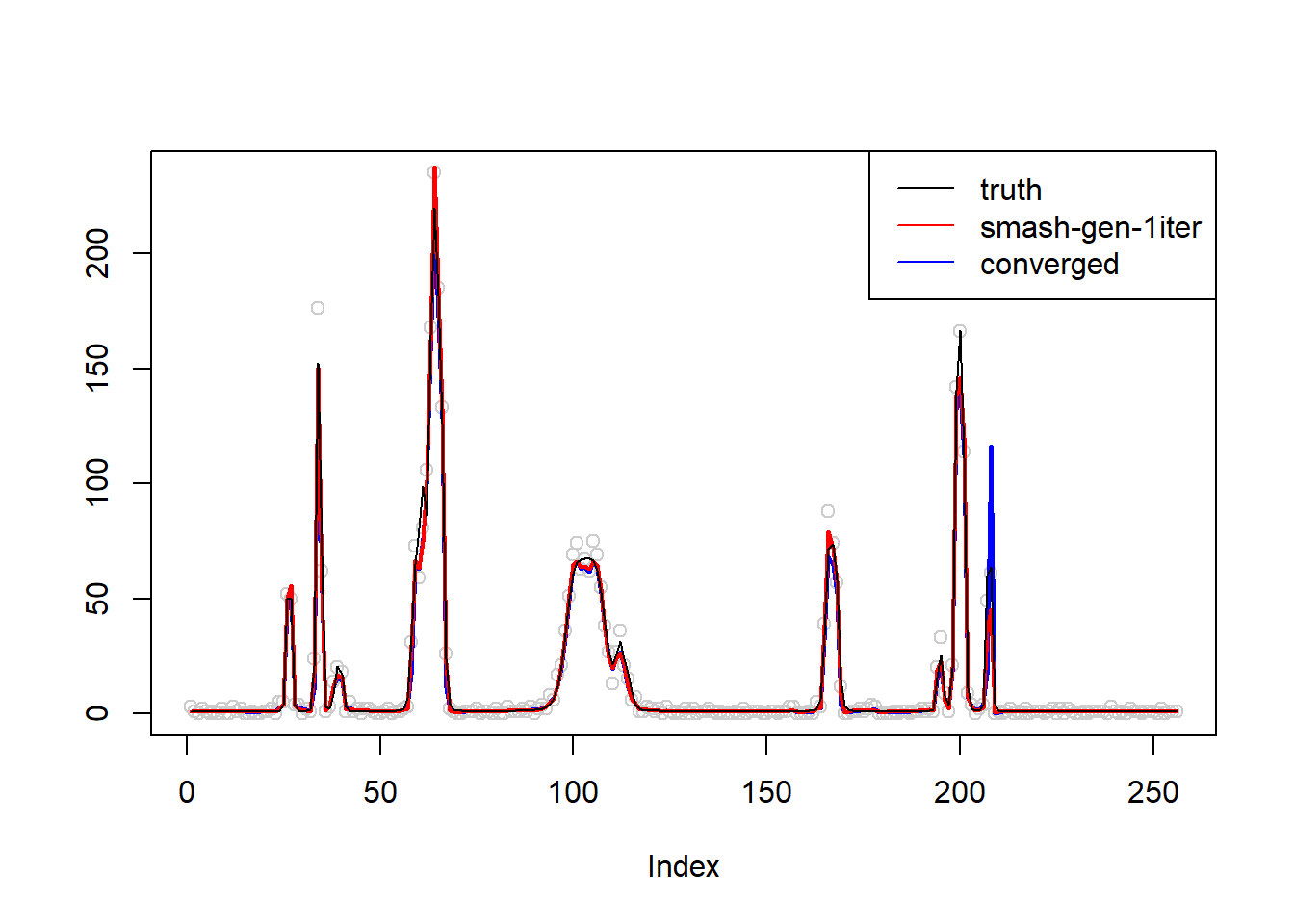

\(\sigma=0.1\)

simu.out=simu_study(m,0.1)
simu.out.conv=simu_study(m,0.1,niter=30)
#par(mfrow = c(1,2))

plot(simu.out$x,col = "gray80" ,ylab = '')
lines(simu.out.conv$smash.gen.out, col = "blue", lwd = 2)
lines(simu.out$smash.gen.out, col = "red", lwd = 2)
lines(exp(m))
legend("topright", # places a legend at the appropriate place
       c("truth","smash-gen-1iter","converged"), # puts text in the legend
       lty=c(1,1,1), # gives the legend appropriate symbols (lines)
       lwd=c(1,1,1),
       cex = 1,
       col=c("black","red", "blue"))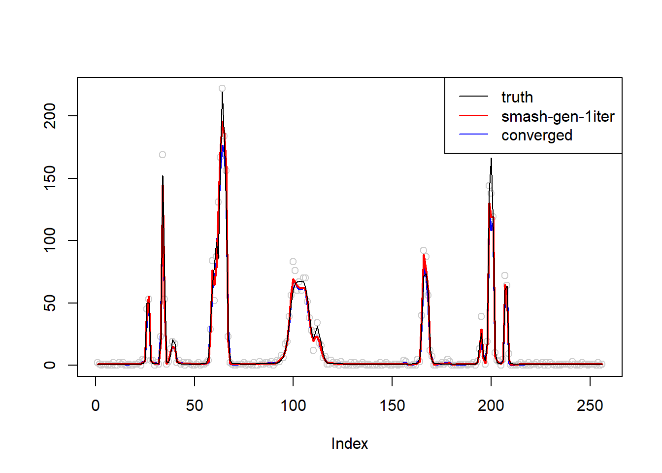

\(\sigma=0.5\)

simu.out=simu_study(m,0.5)
simu.out.conv=simu_study(m,0.5,niter=30)
#par(mfrow = c(1,2))

plot(simu.out$x,col = "gray80" ,ylab = '')
lines(simu.out.conv$smash.gen.out, col = "blue", lwd = 2)
lines(simu.out$smash.gen.out, col = "red", lwd = 2)
lines(exp(m))
legend("topright", # places a legend at the appropriate place
       c("truth","smash-gen-1iter","converged"), # puts text in the legend
       lty=c(1,1,1), # gives the legend appropriate symbols (lines)
       lwd=c(1,1,1),
       cex = 1,
       col=c("black","red", "blue"))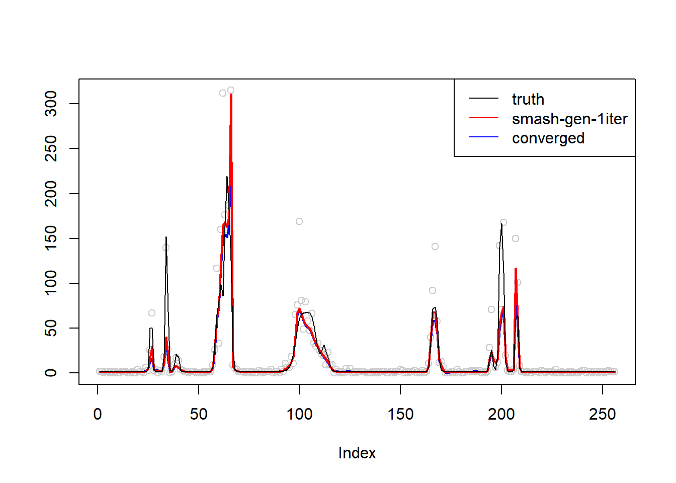

\(\sigma=1\)

simu.out=simu_study(m,1)
simu.out.conv=simu_study(m,1,niter=30)
#par(mfrow = c(1,2))

plot(simu.out$x,col = "gray80" ,ylab = '')
lines(simu.out.conv$smash.gen.out, col = "blue", lwd = 2)
lines(simu.out$smash.gen.out, col = "red", lwd = 2)
lines(exp(m))
legend("topright", # places a legend at the appropriate place
       c("truth","smash-gen-1iter","converged"), # puts text in the legend
       lty=c(1,1,1), # gives the legend appropriate symbols (lines)
       lwd=c(1,1,1),
       cex = 1,
       col=c("black","red", "blue"))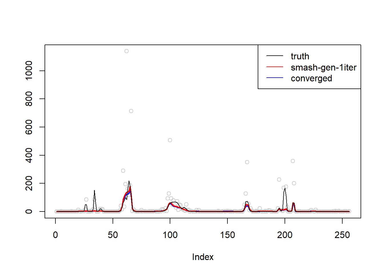

Simulation 5: Sin curve Poisson nugget

\(\sigma=0.01\)

m = seq(-pi,pi,length.out = 256)
m = 2*(sin(m)+1)
simu.out=simu_study(m,0.01)
simu.out.conv=simu_study(m,0.01,niter=30)
#par(mfrow = c(1,2))

plot(simu.out$x,col = "gray80" ,ylab = '')
lines(simu.out.conv$smash.gen.out, col = "blue", lwd = 2)
lines(simu.out$smash.gen.out, col = "red", lwd = 2)
lines(exp(m))
legend("topleft", # places a legend at the appropriate place
       c("truth","smash-gen-1iter","converged"), # puts text in the legend
       lty=c(1,1,1), # gives the legend appropriate symbols (lines)
       lwd=c(1,1,1),
       cex = 1,
       col=c("black","red", "blue"))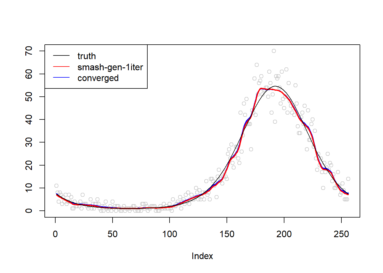

\(\sigma=0.1\)

simu.out=simu_study(m,0.1)
simu.out.conv=simu_study(m,0.1,niter=30)
#par(mfrow = c(1,2))

plot(simu.out$x,col = "gray80" ,ylab = '')
lines(simu.out.conv$smash.gen.out, col = "blue", lwd = 2)
lines(simu.out$smash.gen.out, col = "red", lwd = 2)
lines(exp(m))
legend("topleft", # places a legend at the appropriate place
       c("truth","smash-gen-1iter","converged"), # puts text in the legend
       lty=c(1,1,1), # gives the legend appropriate symbols (lines)
       lwd=c(1,1,1),
       cex = 1,
       col=c("black","red", "blue"))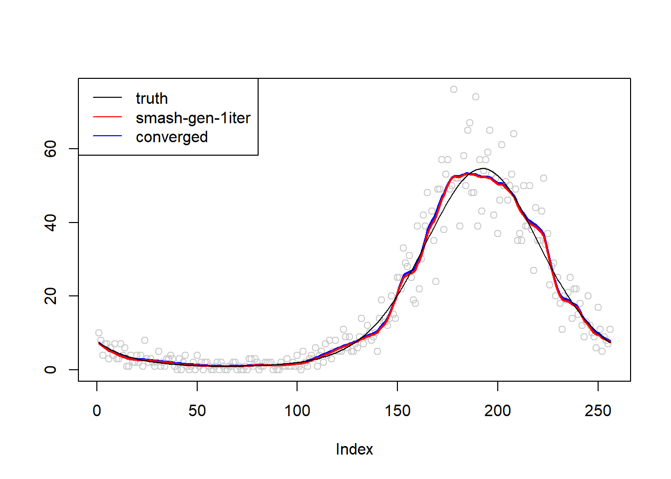

\(\sigma=0.5\)

simu.out=simu_study(m,0.5)
simu.out.conv=simu_study(m,0.5,niter=30)
#par(mfrow = c(1,2))

plot(simu.out$x,col = "gray80" ,ylab = '')
lines(simu.out.conv$smash.gen.out, col = "blue", lwd = 2)
lines(simu.out$smash.gen.out, col = "red", lwd = 2)
lines(exp(m))
legend("topleft", # places a legend at the appropriate place
       c("truth","smash-gen-1iter","converged"), # puts text in the legend
       lty=c(1,1,1), # gives the legend appropriate symbols (lines)
       lwd=c(1,1,1),
       cex = 1,
       col=c("black","red", "blue"))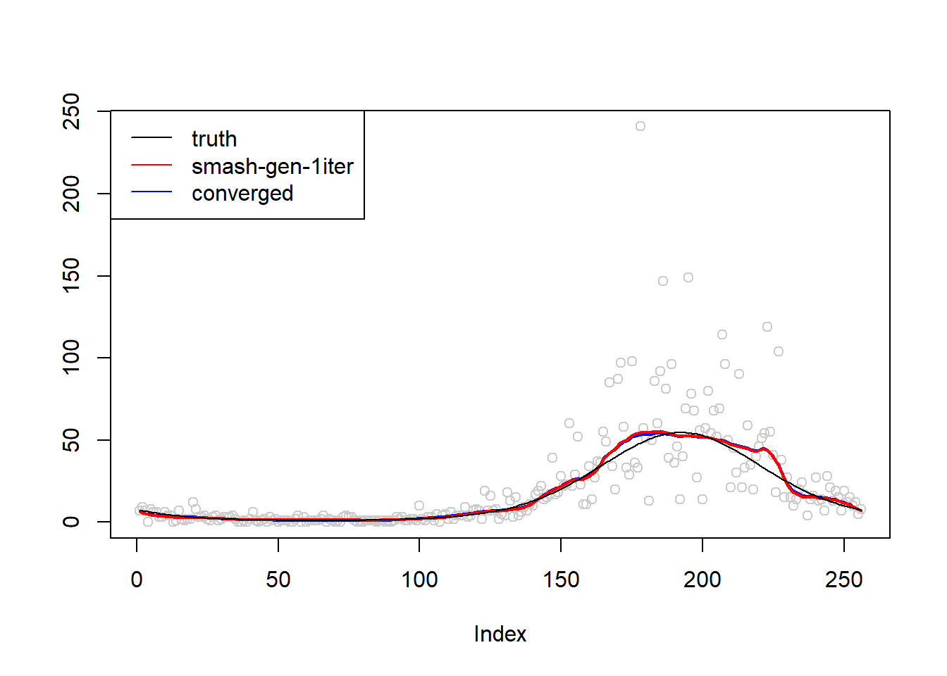

\(\sigma=1\)

simu.out=simu_study(m,1)
simu.out.conv=simu_study(m,1,niter=30)
#par(mfrow = c(1,2))

plot(simu.out$x,col = "gray80" ,ylab = '')
lines(simu.out.conv$smash.gen.out, col = "blue", lwd = 2)
lines(simu.out$smash.gen.out, col = "red", lwd = 2)
lines(exp(m))
legend("topleft", # places a legend at the appropriate place
       c("truth","smash-gen-1iter","converged"), # puts text in the legend
       lty=c(1,1,1), # gives the legend appropriate symbols (lines)
       lwd=c(1,1,1),
       cex = 1,
       col=c("black","red", "blue"))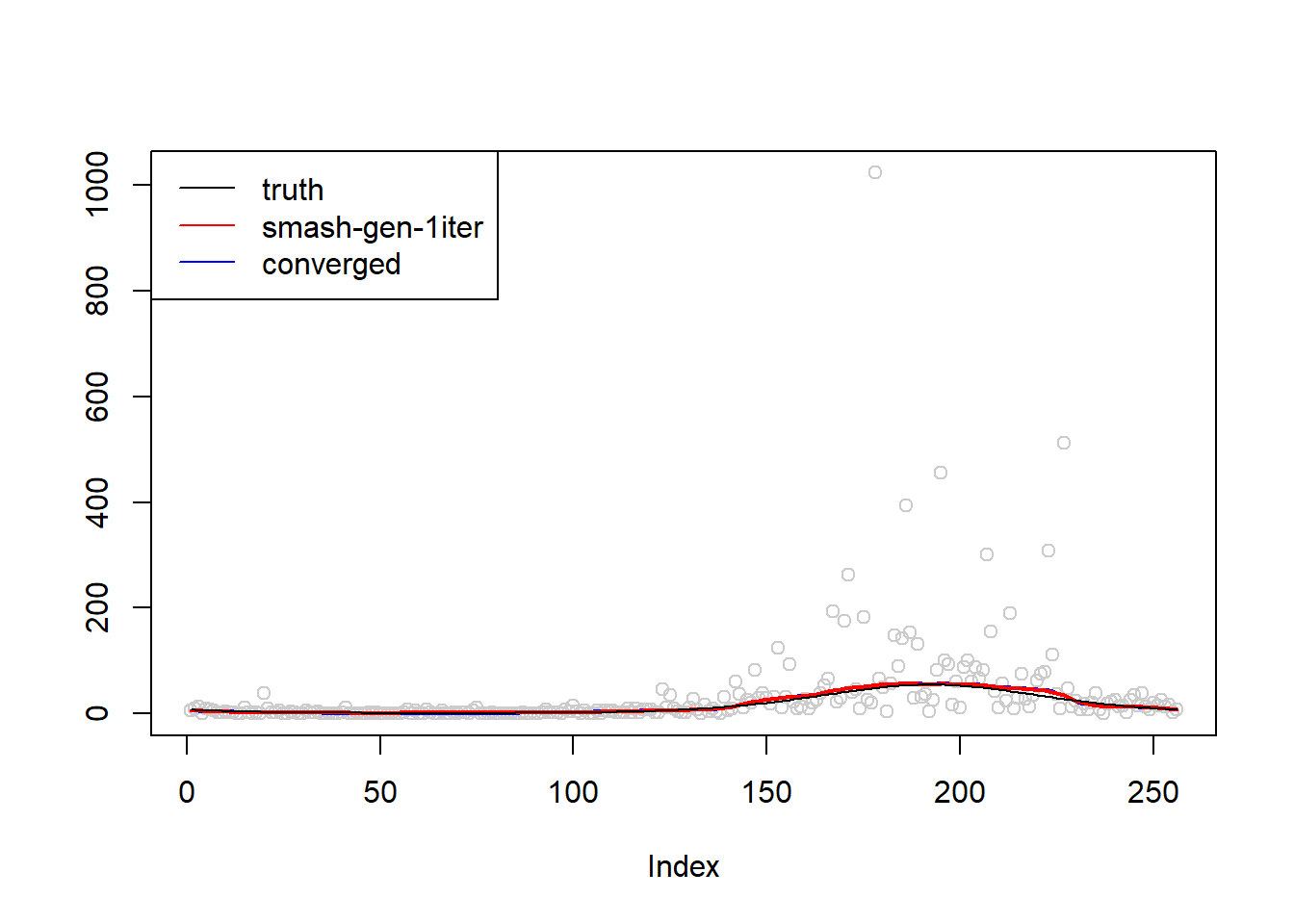

Summary

By applying ash to Poisson data first and expanding around the estimated posterior mean, the performance of 1 iteration algorithm is greatly improved - actually from the above plots, it is almost the same as converged version.

Session information

sessionInfo()

R version 3.4.0 (2017-04-21)
Platform: x86_64-w64-mingw32/x64 (64-bit)
Running under: Windows 10 x64 (build 16299)

Matrix products: default

locale:
[1] LC_COLLATE=English_United States.1252 
[2] LC_CTYPE=English_United States.1252   
[3] LC_MONETARY=English_United States.1252
[4] LC_NUMERIC=C                          
[5] LC_TIME=English_United States.1252    

attached base packages:
[1] stats     graphics  grDevices utils     datasets  methods   base     

other attached packages:
[1] ashr_2.2-7   smashr_1.1-1

loaded via a namespace (and not attached):
 [1] Rcpp_0.12.16        knitr_1.20          whisker_0.3-2      
 [4] magrittr_1.5        workflowr_1.0.1     REBayes_1.3        
 [7] MASS_7.3-47         pscl_1.4.9          doParallel_1.0.11  
[10] SQUAREM_2017.10-1   lattice_0.20-35     foreach_1.4.3      
[13] stringr_1.3.0       caTools_1.17.1      tools_3.4.0        
[16] parallel_3.4.0      grid_3.4.0          data.table_1.10.4-3
[19] R.oo_1.21.0         git2r_0.21.0        iterators_1.0.8    
[22] htmltools_0.3.5     assertthat_0.2.0    yaml_2.1.19        
[25] rprojroot_1.3-2     digest_0.6.13       Matrix_1.2-9       
[28] bitops_1.0-6        codetools_0.2-15    R.utils_2.6.0      
[31] evaluate_0.10       rmarkdown_1.8       wavethresh_4.6.8   
[34] stringi_1.1.6       compiler_3.4.0      Rmosek_8.0.69      
[37] backports_1.0.5     R.methodsS3_1.7.1   truncnorm_1.0-7

This reproducible R Markdown analysis was created with workflowr 1.0.1

One iteration, ash posterior mean

Dongyue Xie

May 8, 2018

Simulation 1: Constant trend Poisson nugget

\(\sigma=0.01\)

\(\sigma=0.1\)

\(\sigma=0.5\)

\(\sigma=1\)

Simulation 2: Step trend

\(\sigma=0.01\)

\(\sigma=0.1\)

\(\sigma=0.5\)

\(\sigma=1\)

Simulation 3: Oscillating Poisson nugget

\(\sigma=0.01\)

\(\sigma=0.1\)

\(\sigma=0.5\)

\(\sigma=1\)

Simulation 4: Bumps

\(\sigma=0.01\)

\(\sigma=0.1\)

\(\sigma=0.5\)

\(\sigma=1\)

Simulation 5: Sin curve Poisson nugget

\(\sigma=0.01\)

\(\sigma=0.1\)

\(\sigma=0.5\)

\(\sigma=1\)

Summary

Session information