Binomial wavelet smoothing
Dongyue Xie
May 12, 2018
Last updated: 2018-05-17
workflowr checks: (Click a bullet for more information)-
✔ R Markdown file: up-to-date
Great! Since the R Markdown file has been committed to the Git repository, you know the exact version of the code that produced these results.
-
✔ Environment: empty
Great job! The global environment was empty. Objects defined in the global environment can affect the analysis in your R Markdown file in unknown ways. For reproduciblity it’s best to always run the code in an empty environment.
-
✔ Seed:
set.seed(20180501)The command
set.seed(20180501)was run prior to running the code in the R Markdown file. Setting a seed ensures that any results that rely on randomness, e.g. subsampling or permutations, are reproducible. -
✔ Session information: recorded
Great job! Recording the operating system, R version, and package versions is critical for reproducibility.
-
Great! You are using Git for version control. Tracking code development and connecting the code version to the results is critical for reproducibility. The version displayed above was the version of the Git repository at the time these results were generated.✔ Repository version: 3c0ccfd
Note that you need to be careful to ensure that all relevant files for the analysis have been committed to Git prior to generating the results (you can usewflow_publishorwflow_git_commit). workflowr only checks the R Markdown file, but you know if there are other scripts or data files that it depends on. Below is the status of the Git repository when the results were generated:
Note that any generated files, e.g. HTML, png, CSS, etc., are not included in this status report because it is ok for generated content to have uncommitted changes.Ignored files: Ignored: .Rhistory Ignored: .Rproj.user/ Ignored: log/ Untracked files: Untracked: analysis/binom.Rmd Untracked: analysis/overdis.Rmd Untracked: analysis/smashtutorial.Rmd Untracked: docs/figure/smashtutorial.Rmd/ Unstaged changes: Modified: analysis/ashpmean.Rmd Modified: analysis/nugget.Rmd
Expand here to see past versions:
Algorithm
Let \(X_t\) be a Binomial observation with number of trials \(n_t\), \(t=1,2,\dots,T\).
- Apply
ashto binomial data \((X_t, n_t)\) and obtain the posterior mean \(\hat p=E(p|X,n)\), \(\hat p\in R^T\). - Let \(s_t=\frac{1}{n_t\hat p_t(1-\hat p_t)}\) and \(Y_t=\log\frac{\hat p_t}{1-\hat p_t}+\frac{X_t/n_t-\hat p_t}{n_t\hat p_t(1-\hat p_t)}\).
- Apply
smash.gausto \(Y_t\) with standard deviation \(\sqrt(\sigma^2+s_t^2)\) if \(\sigma^2\) is known. If it’s unknown, then either \(\sigma^2\) or \(\sigma^2+s_t^2\) should be estimated first. The output ofsmash.gausis denoted as \(\mu_t\). - Export \(\frac{\exp(\mu_t)}{1+\exp(\mu_t)}\).
Methods for estimating \(\sigma^2\) or \(\sigma^2+s_t^2\) are discussed here.
library(smashrgen)
library(ggplot2)
simu_study=function(p,sigma,ntri,nsimu=100,seed=12345,
                    niter=1,family='DaubExPhase',ashp=TRUE,verbose=FALSE,robust=FALSE,
                    tol=1e-2){
  set.seed(seed)
  #smash.err=c()
  smashgen.err=c()
  smashgen.smashu.err=c()
  #smashgen.mle.err=c()
  n=length(p)
  true.p=exp(p)/(1+exp(p))
  for(k in 1:nsimu){
    ng=rnorm(n,0,sigma)
    m=exp(p+ng)
    q=m/(1+m)
    x=rbinom(n,ntri,q)
    #fit data
    #smash.out=smash.poiss(x)
    smashgen.out=smash_gen(x,dist_family = 'binomial',sigma = sigma,ntri=ntri)
    smashu.out=smash_gen(x,dist_family = 'binomial',y_var_est = 'smashu',ntri=ntri)
    #mle.out=smash_gen(x,dist_family = 'poisson',y_var_est = 'mle')
    #smash.err[k]=mse(exp(m),smash.out)
    smashgen.err[k]=mse(true.p,smashgen.out)
    smashgen.smashu.err[k]=mse(true.p,smashu.out)
    #smashgen.mle.err[k]=mse(exp(m),mle.out)
  }
  return(list(est=list(smashgen.out=smashgen.out,smashu.out=smashu.out,x=x),err=data.frame(smashgen=smashgen.err, smashgen.smashu=smashgen.smashu.err)))
}
Constant trend
\(\sigma=0.1\)
p=rep(0,128)
set.seed(111)
ntri=rpois(128,30)
result=simu_study(p,0.1,ntri)
par(mfrow=c(1,2))
plot(result$est$x/ntri,col='gray80',ylab='',main='smashgen: known variance')
lines(exp(p)/(1+exp(p)),col=1)
lines(result$est$smashgen.out,col=4)
legend("topright", # places a legend at the appropriate place
       c("truth","smashgen"), # puts text in the legend
       lty=c(1,1), # gives the legend appropriate symbols (lines)
       lwd=c(1,1),
       cex = 1,
       col=c("black","blue"))
plot(result$est$x/ntri,col='gray80',ylab='',main='smashgen: unknown variance')
lines(exp(p)/(1+exp(p)),col=1)
lines(result$est$smashu.out,col=4)
legend("topright", # places a legend at the appropriate place
       c("truth","smashgen"), # puts text in the legend
       lty=c(1,1), # gives the legend appropriate symbols (lines)
       lwd=c(1,1),
       cex = 1,
       col=c("black","blue"))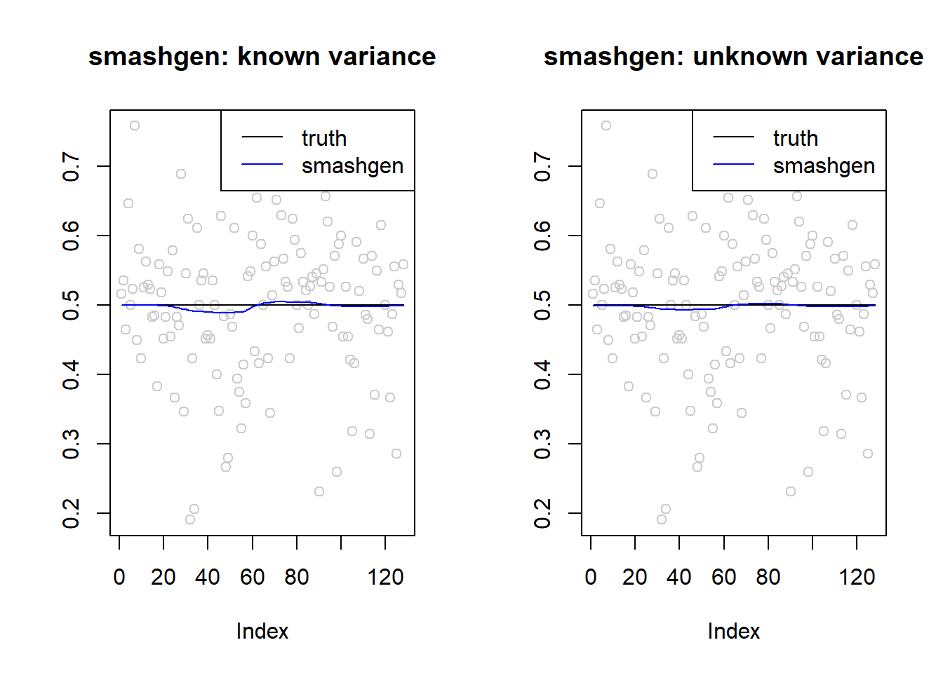
mean(result$err$smashgen)[1] 8.957221e-05mean(result$err$smashgen.smashu)[1] 9.913624e-05ggplot(df2gg(result$err),aes(x=method,y=MSE))+geom_boxplot(aes(fill=method))+labs(x='')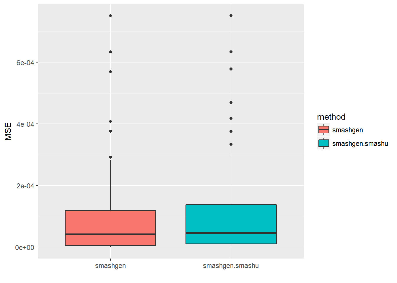
\(\sigma=1\)
result=simu_study(p,1,ntri)
par(mfrow=c(1,2))
plot(result$est$x/ntri,col='gray80',ylab='',main='smashgen: known variance')
lines(exp(p)/(1+exp(p)),col=1)
lines(result$est$smashgen.out,col=4)
plot(result$est$x/ntri,col='gray80',ylab='',main='smashgen: unknown variance')
lines(exp(p)/(1+exp(p)),col=1)
lines(result$est$smashu.out,col=4)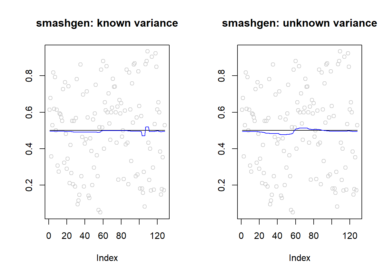
mean(result$err$smashgen)[1] 0.0007841879mean(result$err$smashgen.smashu)[1] 0.0008206814ggplot(df2gg(result$err),aes(x=method,y=MSE))+geom_boxplot(aes(fill=method))+labs(x='')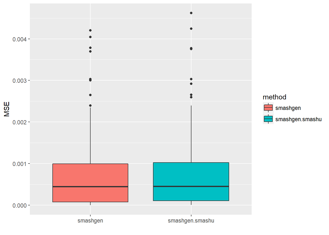
\(\sigma=1\), small prob
p=rep(-3,128)
result=simu_study(p,1,ntri)
par(mfrow=c(1,2))
plot(result$est$x/ntri,col='gray80',ylab='',main='smashgen: known variance')
lines(exp(p)/(1+exp(p)),col=1)
lines(result$est$smashgen.out,col=4)
plot(result$est$x/ntri,col='gray80',ylab='',main='smashgen: unknown variance')
lines(exp(p)/(1+exp(p)),col=1)
lines(result$est$smashu.out,col=4)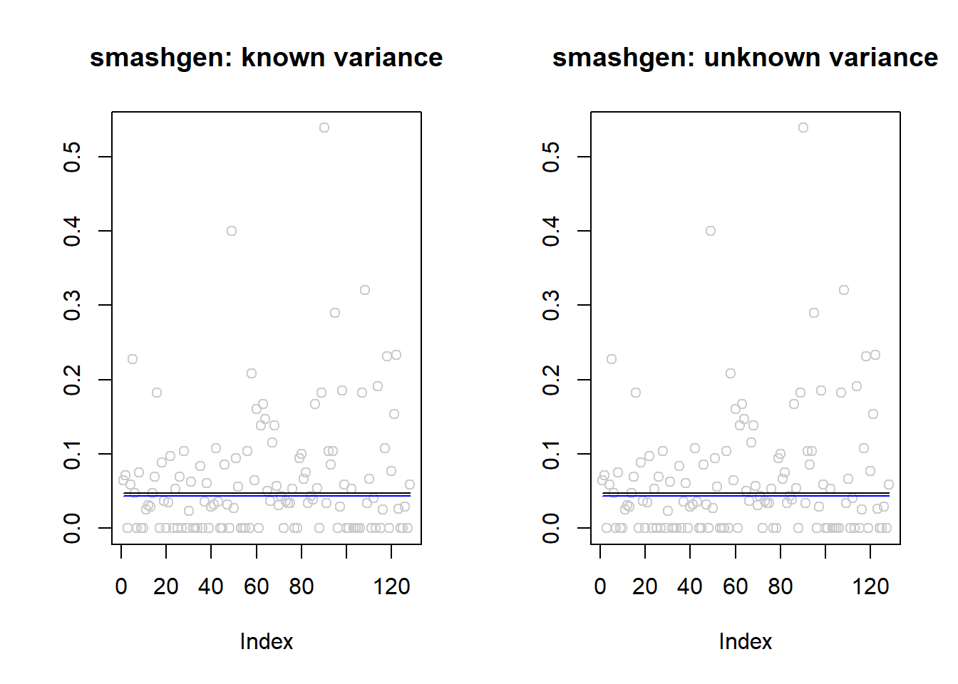
mean(result$err$smashgen)[1] 2.175465e-05mean(result$err$smashgen.smashu)[1] 2.726665e-05ggplot(df2gg(result$err),aes(x=method,y=MSE))+geom_boxplot(aes(fill=method))+labs(x='')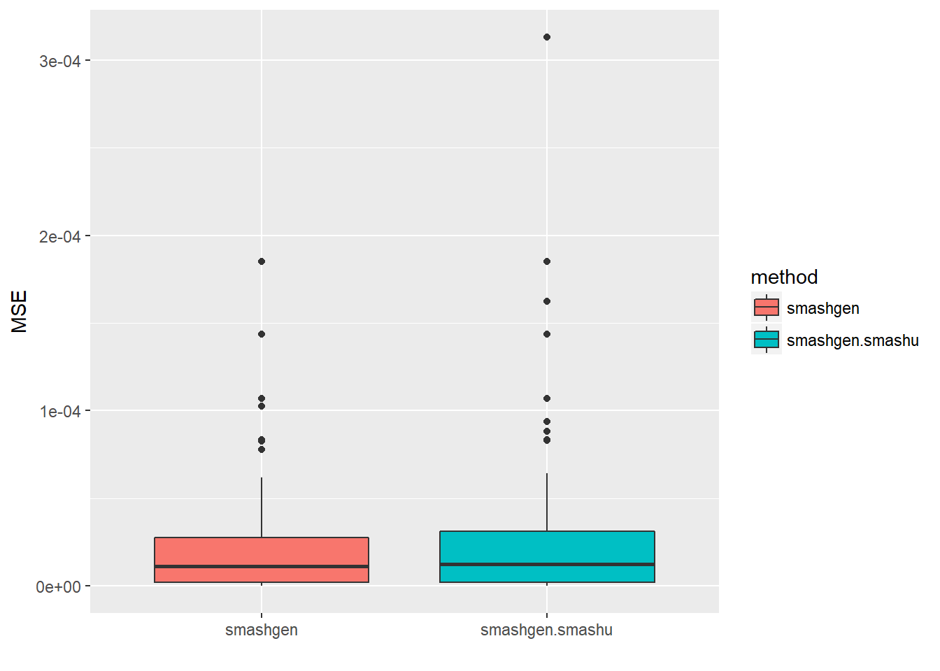
Step trend
\(\sigma=0.1\)
p=c(rep(-2,128), rep(0, 128), rep(2, 128), rep(-2, 128))
set.seed(111)
ntri=rpois(512,30)
result=simu_study(p,0.1,ntri)

par(mfrow=c(1,2))
plot(result$est$x/ntri,col='gray80',ylab='',main='smashgen: known variance')
lines(exp(p)/(1+exp(p)),col=1)
lines(result$est$smashgen.out,col=4)
plot(result$est$x/ntri,col='gray80',ylab='',main='smashgen: unknown variance')
lines(exp(p)/(1+exp(p)),col=1)
lines(result$est$smashu.out,col=4)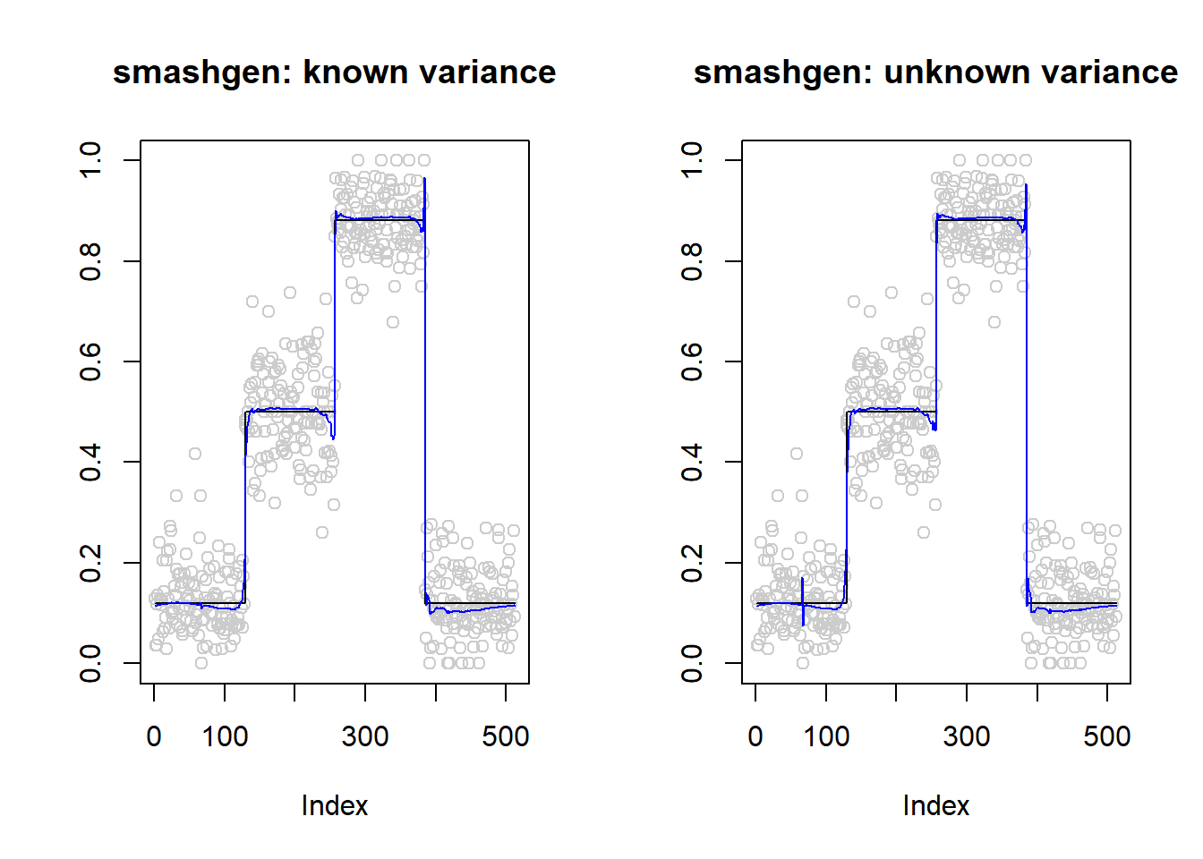
mean(result$err$smashgen)[1] 0.0003595882mean(result$err$smashgen.smashu)[1] 0.0004350061ggplot(df2gg(result$err),aes(x=method,y=MSE))+geom_boxplot(aes(fill=method))+labs(x='')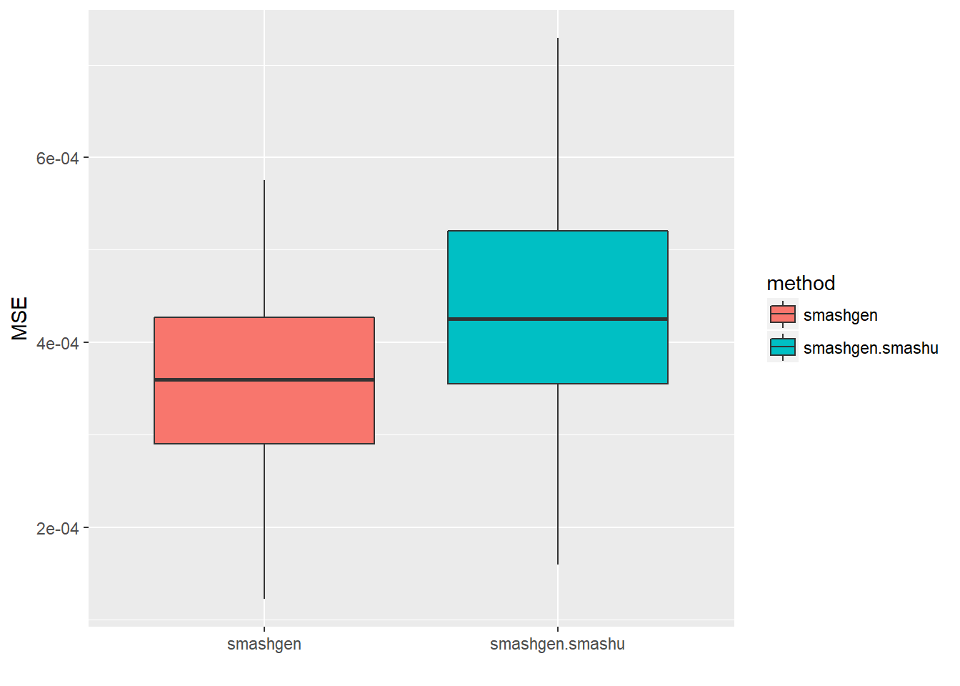
\(\sigma=1\)
p=c(rep(-2,128), rep(0, 128), rep(2, 128), rep(-2, 128))
set.seed(111)
ntri=rpois(512,30)
result=simu_study(p,1,ntri)

par(mfrow=c(1,2))
plot(result$est$x/ntri,col='gray80',ylab='',main='smashgen: known variance')
lines(exp(p)/(1+exp(p)),col=1)
lines(result$est$smashgen.out,col=4)
plot(result$est$x/ntri,col='gray80',ylab='',main='smashgen: unknown variance')
lines(exp(p)/(1+exp(p)),col=1)
lines(result$est$smashu.out,col=4)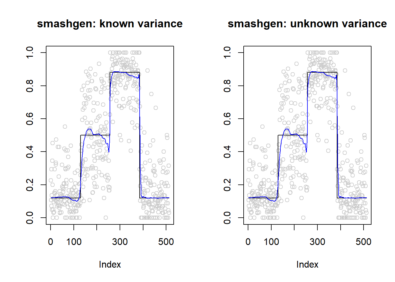
mean(result$err$smashgen)[1] 0.001850991mean(result$err$smashgen.smashu)[1] 0.001842285ggplot(df2gg(result$err),aes(x=method,y=MSE))+geom_boxplot(aes(fill=method))+labs(x='')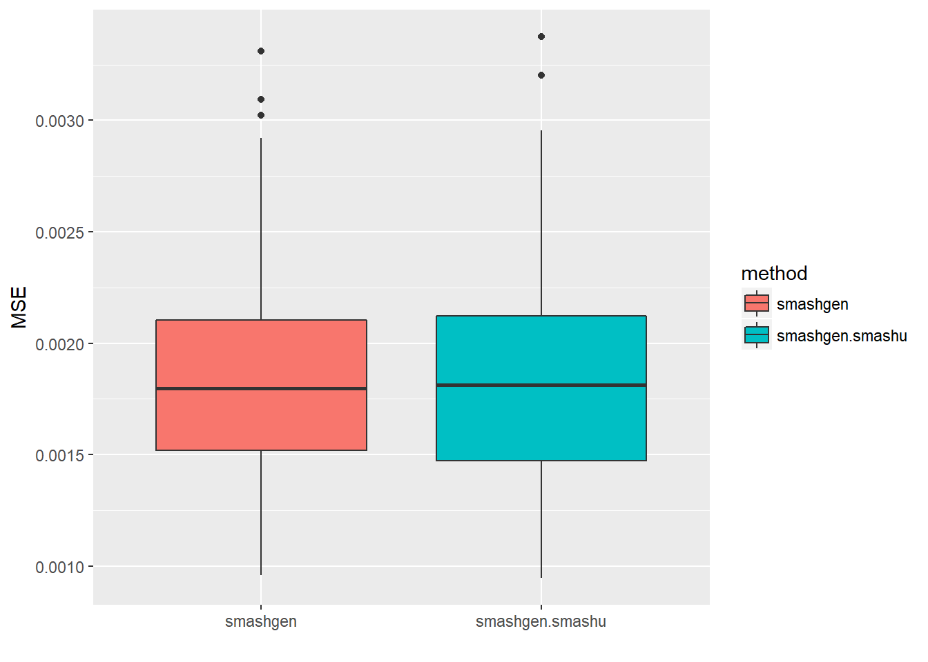
\(\sigma=1\), more variant ntri
p=c(rep(-2,128), rep(0, 128), rep(2, 128), rep(-2, 128))
set.seed(111)
ntri=rpois(512,50)-20
result=simu_study(p,1,ntri)

par(mfrow=c(1,2))
plot(result$est$x/ntri,col='gray80',ylab='',main='smashgen: known variance')
lines(exp(p)/(1+exp(p)),col=1)
lines(result$est$smashgen.out,col=4)
plot(result$est$x/ntri,col='gray80',ylab='',main='smashgen: unknown variance')
lines(exp(p)/(1+exp(p)),col=1)
lines(result$est$smashu.out,col=4)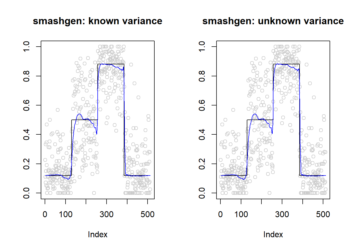
mean(result$err$smashgen)[1] 0.001875976mean(result$err$smashgen.smashu)[1] 0.001847042ggplot(df2gg(result$err),aes(x=method,y=MSE))+geom_boxplot(aes(fill=method))+labs(x='')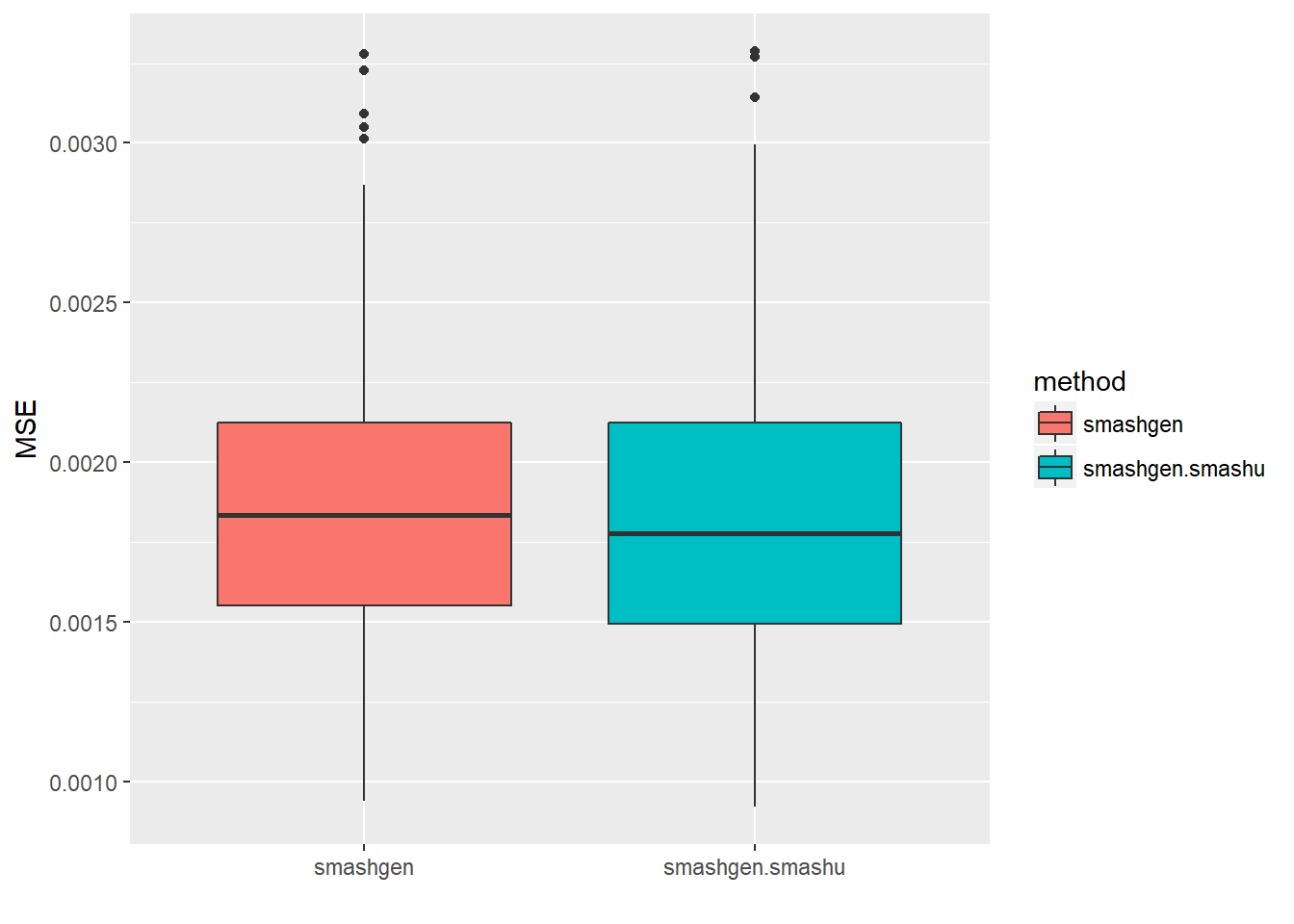
Bumps
\(\sigma=0.1\)
m=seq(0,1,length.out = 256)
h = c(4, 5, 3, 4, 5, 4.2, 2.1, 4.3, 3.1, 5.1, 4.2)
w = c(0.005, 0.005, 0.006, 0.01, 0.01, 0.03, 0.01, 0.01, 0.005,0.008,0.005)
t=c(.1,.13,.15,.23,.25,.4,.44,.65,.76,.78,.81)
f = c()
for(i in 1:length(m)){
  f[i]=sum(h*(1+((m[i]-t)/w)^4)^(-1))
}
p=f-3

set.seed(111)
ntri=rpois(256,30)
result=simu_study(p,0.1,ntri)

par(mfrow=c(1,2))
plot(result$est$x/ntri,col='gray80',ylab='',main='smashgen: known variance')
lines(exp(p)/(1+exp(p)),col=1)
lines(result$est$smashgen.out,col=4)
plot(result$est$x/ntri,col='gray80',ylab='',main='smashgen: unknown variance')
lines(exp(p)/(1+exp(p)),col=1)
lines(result$est$smashu.out,col=4)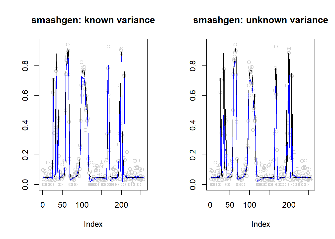
mean(result$err$smashgen)[1] 0.001821751mean(result$err$smashgen.smashu)[1] 0.005024706ggplot(df2gg(result$err),aes(x=method,y=MSE))+geom_boxplot(aes(fill=method))+labs(x='')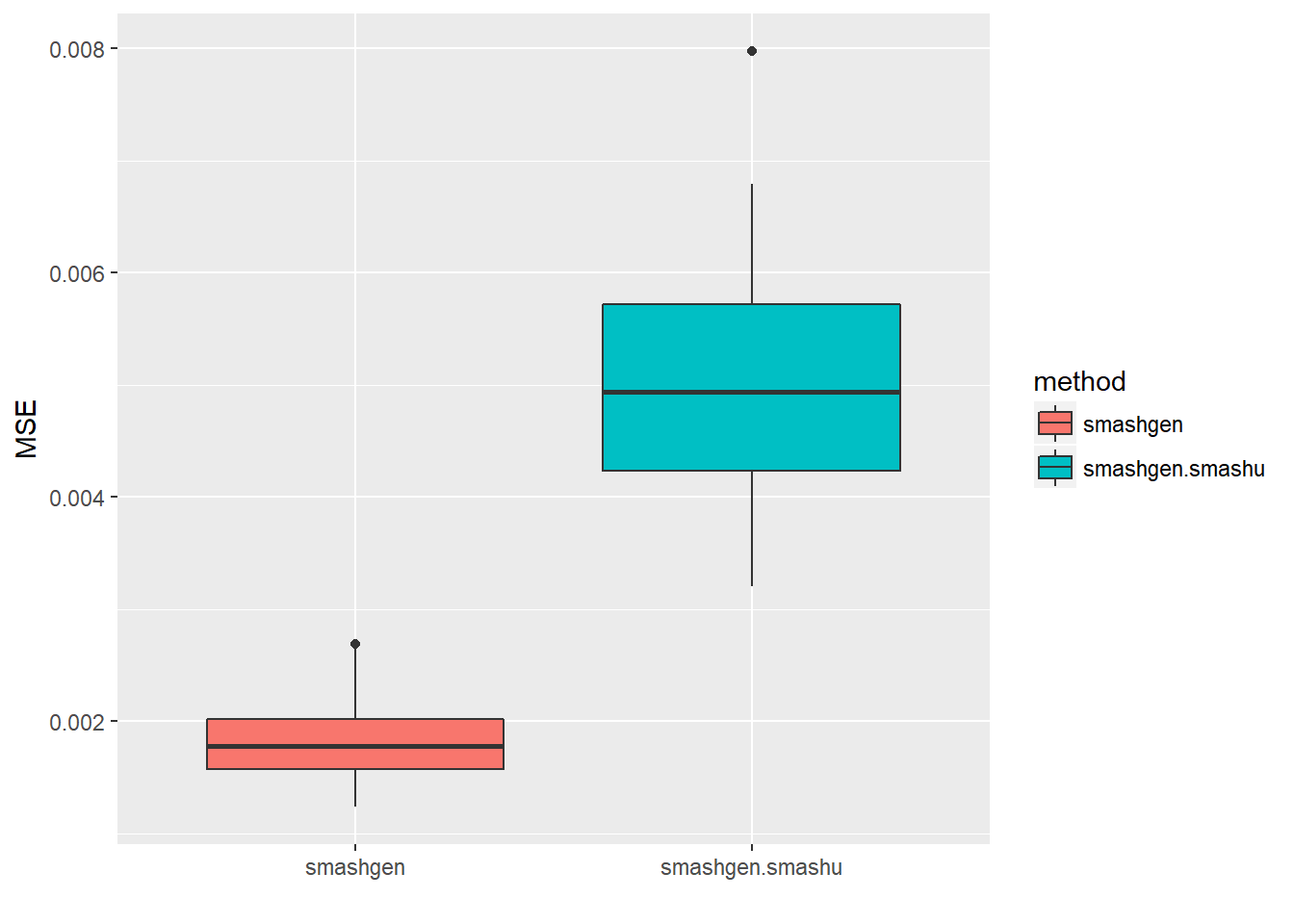
\(\sigma=1\)
set.seed(111)
ntri=rpois(256,30)
result=simu_study(p,1,ntri)

par(mfrow=c(1,2))
plot(result$est$x/ntri,col='gray80',ylab='',main='smashgen: known variance')
lines(exp(p)/(1+exp(p)),col=1)
lines(result$est$smashgen.out,col=4)
plot(result$est$x/ntri,col='gray80',ylab='',main='smashgen: unknown variance')
lines(exp(p)/(1+exp(p)),col=1)
lines(result$est$smashu.out,col=4)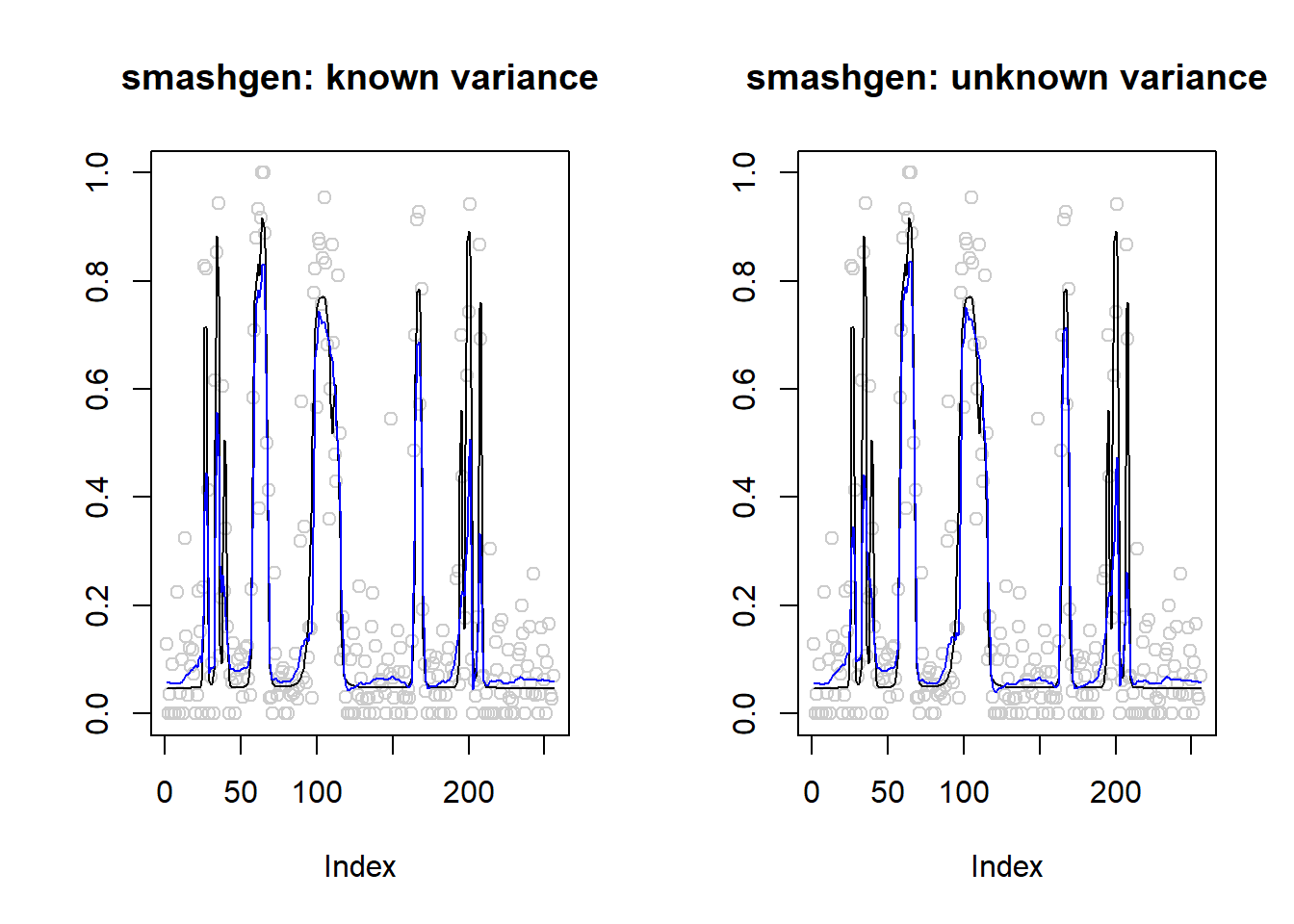
mean(result$err$smashgen)[1] 0.0124867mean(result$err$smashgen.smashu)[1] 0.01233137ggplot(df2gg(result$err),aes(x=method,y=MSE))+geom_boxplot(aes(fill=method))+labs(x='')
\(\sigma=1\), more variant ntri
set.seed(111)
ntri=rpois(256,50)-20
result=simu_study(p,1,ntri)

par(mfrow=c(1,2))
plot(result$est$x/ntri,col='gray80',ylab='',main='smashgen: known variance')
lines(exp(p)/(1+exp(p)),col=1)
lines(result$est$smashgen.out,col=4)
plot(result$est$x/ntri,col='gray80',ylab='',main='smashgen: unknown variance')
lines(exp(p)/(1+exp(p)),col=1)
lines(result$est$smashu.out,col=4)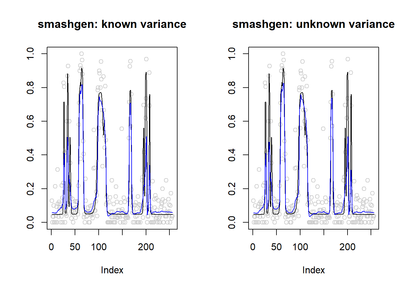
mean(result$err$smashgen)[1] 0.01249222mean(result$err$smashgen.smashu)[1] 0.01226534ggplot(df2gg(result$err),aes(x=method,y=MSE))+geom_boxplot(aes(fill=method))+labs(x='')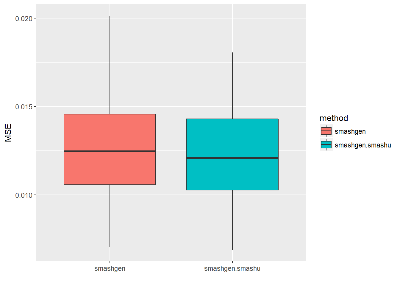
\(\sigma=1\), smaller ntri
set.seed(111)
ntri=rpois(256,20)-9
result=simu_study(p,1,ntri)

par(mfrow=c(1,2))
plot(result$est$x/ntri,col='gray80',ylab='',main='smashgen: known variance')
lines(exp(p)/(1+exp(p)),col=1)
lines(result$est$smashgen.out,col=4)
plot(result$est$x/ntri,col='gray80',ylab='',main='smashgen: unknown variance')
lines(exp(p)/(1+exp(p)),col=1)
lines(result$est$smashu.out,col=4)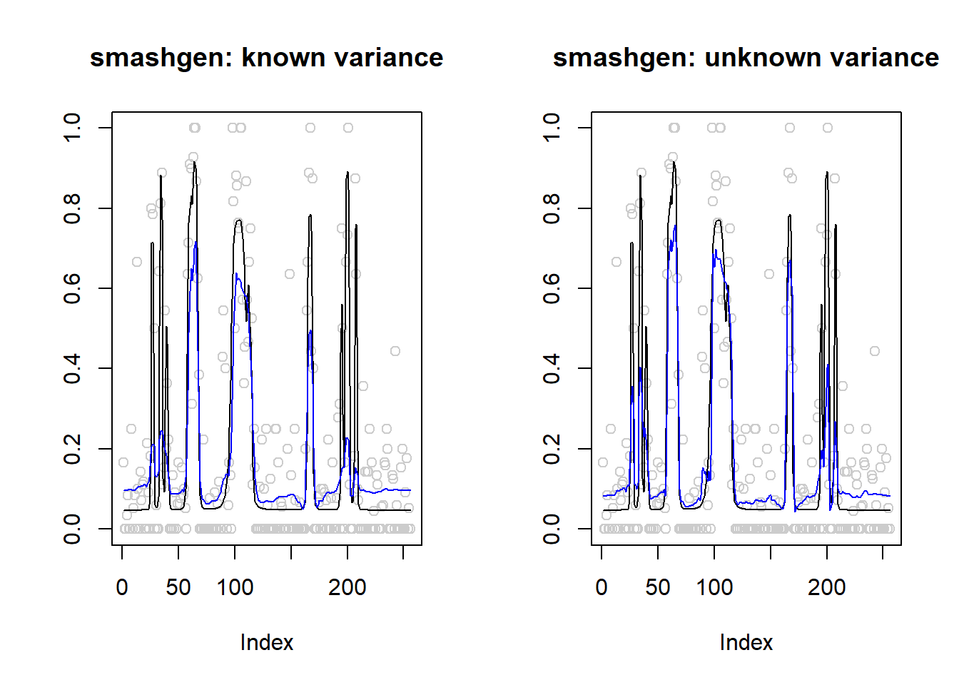
mean(result$err$smashgen)[1] 0.02209255mean(result$err$smashgen.smashu)[1] 0.01565017ggplot(df2gg(result$err),aes(x=method,y=MSE))+geom_boxplot(aes(fill=method))+labs(x='')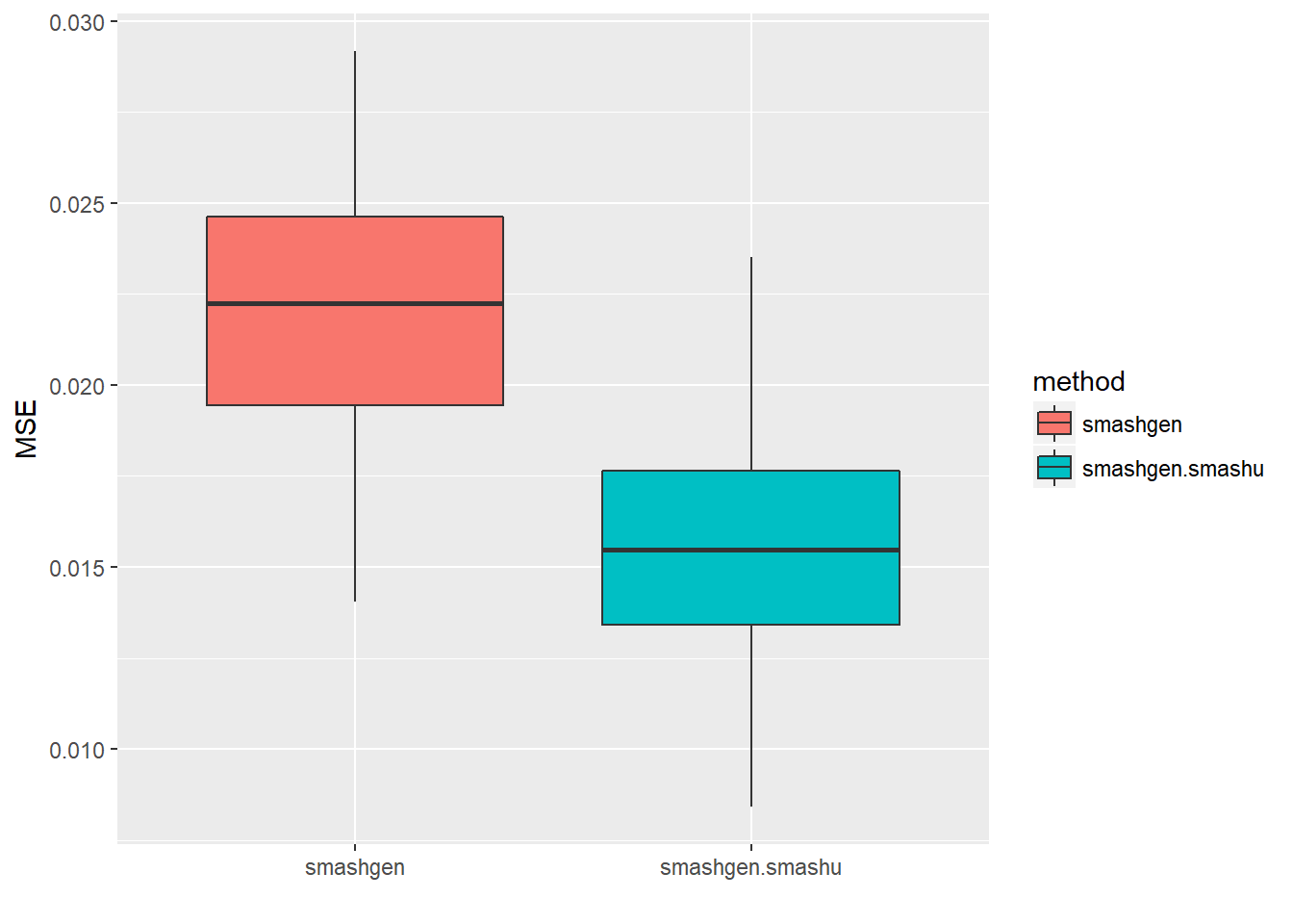
Spike mean
\(\sigma=0.1\)
spike.f = function(x) (0.75 * exp(-500 * (x - 0.23)^2) + 1.5 * exp(-2000 * (x - 0.33)^2) + 3 * exp(-8000 * (x - 0.47)^2) + 2.25 * exp(-16000 *
    (x - 0.69)^2) + 0.5 * exp(-32000 * (x - 0.83)^2))
n = 256
t = 1:n/n
p = spike.f(t)*2-2

set.seed(111)
ntri=rpois(256,20)-9
result=simu_study(p,0.1,ntri)

par(mfrow=c(1,2))
plot(result$est$x/ntri,col='gray80',ylab='',main='smashgen: known variance')
lines(exp(p)/(1+exp(p)),col=1)
lines(result$est$smashgen.out,col=4)
plot(result$est$x/ntri,col='gray80',ylab='',main='smashgen: unknown variance')
lines(exp(p)/(1+exp(p)),col=1)
lines(result$est$smashu.out,col=4)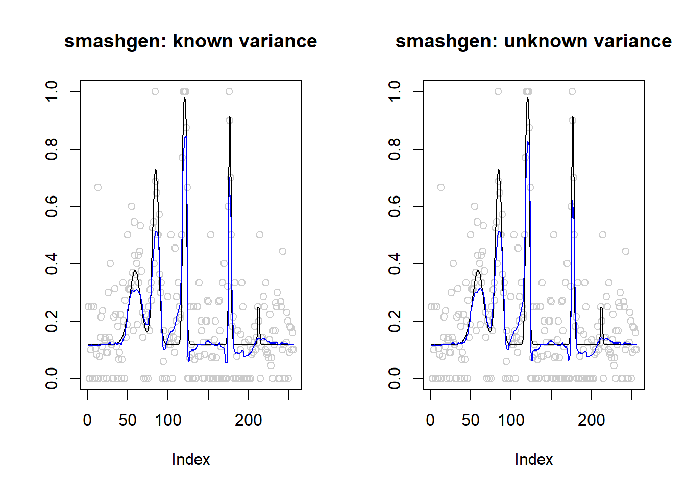
mean(result$err$smashgen)[1] 0.003198372mean(result$err$smashgen.smashu)[1] 0.003931562ggplot(df2gg(result$err),aes(x=method,y=MSE))+geom_boxplot(aes(fill=method))+labs(x='')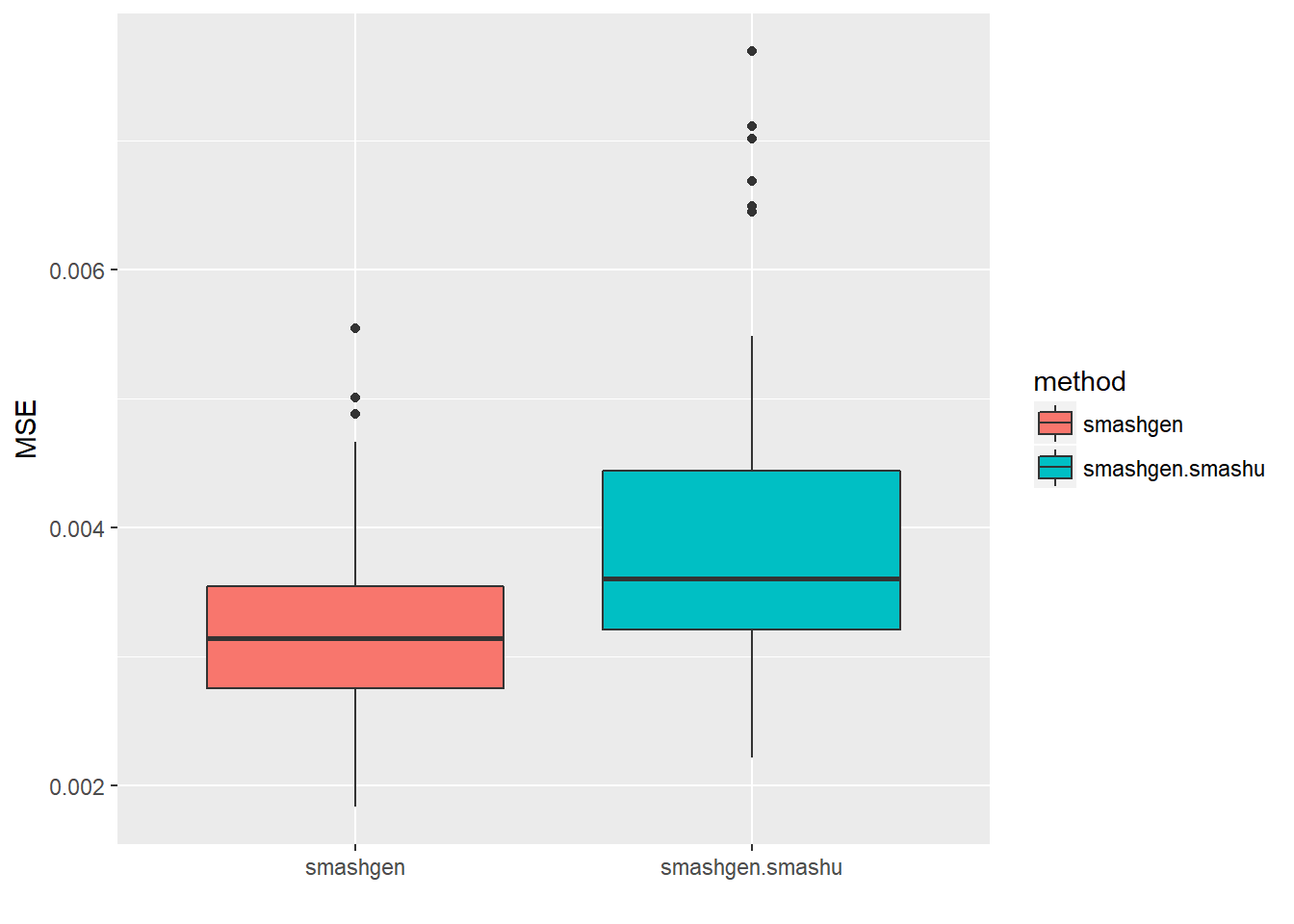
\(\sigma=1\)
set.seed(111)
ntri=rpois(256,20)-9
result=simu_study(p,1,ntri)

par(mfrow=c(1,2))
plot(result$est$x/ntri,col='gray80',ylab='',main='smashgen: known variance')
lines(exp(p)/(1+exp(p)),col=1)
lines(result$est$smashgen.out,col=4)
plot(result$est$x/ntri,col='gray80',ylab='',main='smashgen: unknown variance')
lines(exp(p)/(1+exp(p)),col=1)
lines(result$est$smashu.out,col=4)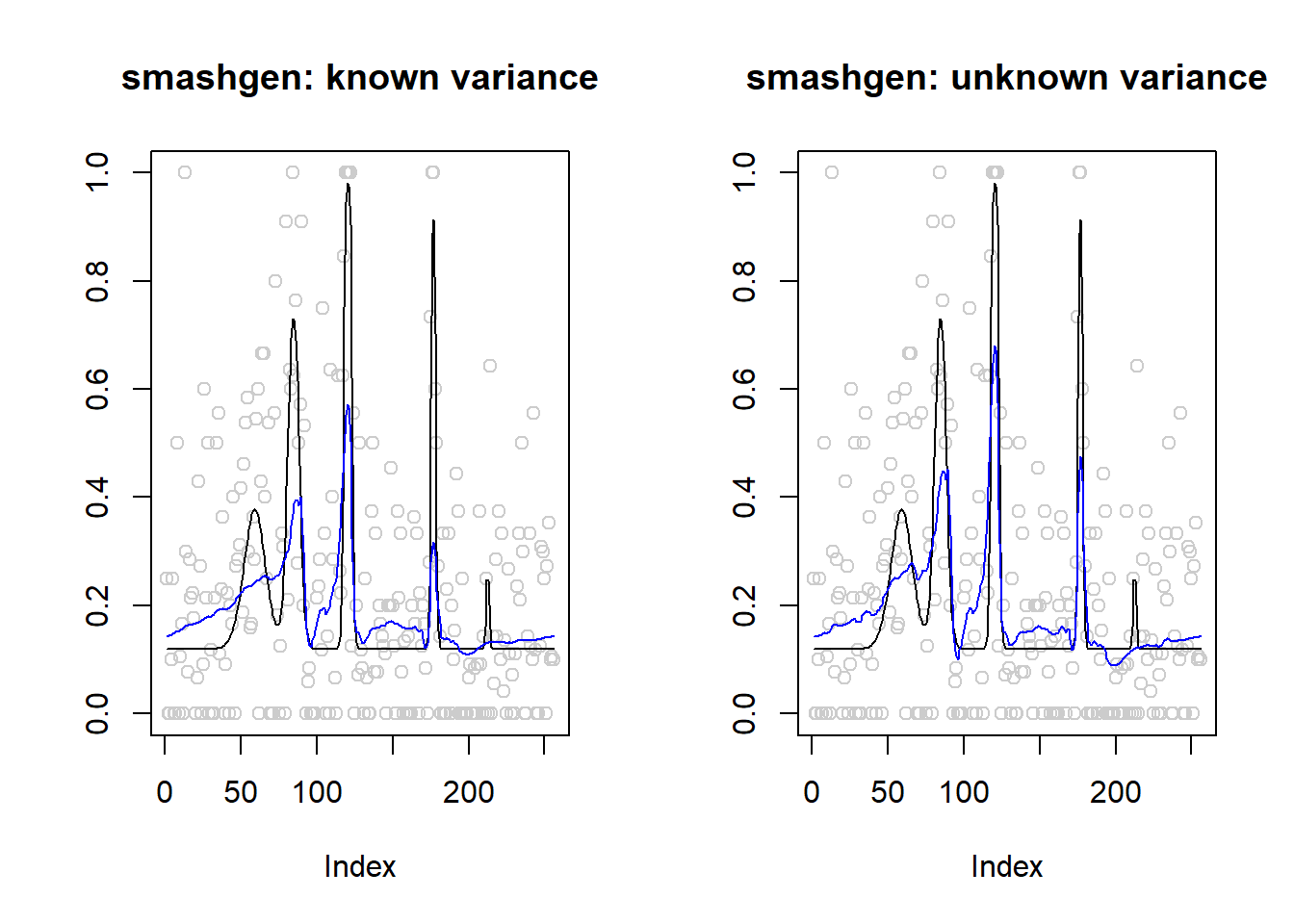
mean(result$err$smashgen)[1] 0.01327303mean(result$err$smashgen.smashu)[1] 0.009787627ggplot(df2gg(result$err),aes(x=method,y=MSE))+geom_boxplot(aes(fill=method))+labs(x='')
Session information
sessionInfo()R version 3.4.0 (2017-04-21)
Platform: x86_64-w64-mingw32/x64 (64-bit)
Running under: Windows 10 x64 (build 16299)
Matrix products: default
locale:
[1] LC_COLLATE=English_United States.1252
[2] LC_CTYPE=English_United States.1252
[3] LC_MONETARY=English_United States.1252
[4] LC_NUMERIC=C
[5] LC_TIME=English_United States.1252
attached base packages:
[1] stats graphics grDevices utils datasets methods base
other attached packages:
[1] ggplot2_2.2.1 smashrgen_0.1.0 wavethresh_4.6.8 MASS_7.3-47
[5] caTools_1.17.1 ashr_2.2-7 smashr_1.1-5
loaded via a namespace (and not attached):
[1] Rcpp_0.12.16 plyr_1.8.4 compiler_3.4.0
[4] git2r_0.21.0 workflowr_1.0.1 R.methodsS3_1.7.1
[7] R.utils_2.6.0 bitops_1.0-6 iterators_1.0.8
[10] tools_3.4.0 digest_0.6.13 tibble_1.3.3
[13] evaluate_0.10 gtable_0.2.0 lattice_0.20-35
[16] rlang_0.1.2 Matrix_1.2-9 foreach_1.4.3
[19] yaml_2.1.19 parallel_3.4.0 stringr_1.3.0
[22] knitr_1.20 REBayes_1.3 rprojroot_1.3-2
[25] grid_3.4.0 data.table_1.10.4-3 rmarkdown_1.8
[28] magrittr_1.5 whisker_0.3-2 backports_1.0.5
[31] scales_0.4.1 codetools_0.2-15 htmltools_0.3.5
[34] assertthat_0.2.0 colorspace_1.3-2 labeling_0.3
[37] stringi_1.1.6 Rmosek_8.0.69 lazyeval_0.2.1
[40] munsell_0.4.3 doParallel_1.0.11 pscl_1.4.9
[43] truncnorm_1.0-7 SQUAREM_2017.10-1 R.oo_1.21.0 This reproducible R Markdown analysis was created with workflowr 1.0.1