Last updated: 2018-05-25

workflowr checks: (Click a bullet for more information)

✔ R Markdown file: up-to-date

Great! Since the R Markdown file has been committed to the Git repository, you know the exact version of the code that produced these results.
✔ Environment: empty

Great job! The global environment was empty. Objects defined in the global environment can affect the analysis in your R Markdown file in unknown ways. For reproduciblity it’s best to always run the code in an empty environment.
✔ Seed: set.seed(20180501)

The command set.seed(20180501) was run prior to running the code in the R Markdown file. Setting a seed ensures that any results that rely on randomness, e.g. subsampling or permutations, are reproducible.
✔ Session information: recorded

Great job! Recording the operating system, R version, and package versions is critical for reproducibility.
✔ Repository version: c89829a
Great! You are using Git for version control. Tracking code development and connecting the code version to the results is critical for reproducibility. The version displayed above was the version of the Git repository at the time these results were generated.

Note that you need to be careful to ensure that all relevant files for the analysis have been committed to Git prior to generating the results (you can use wflow_publish or wflow_git_commit). workflowr only checks the R Markdown file, but you know if there are other scripts or data files that it depends on. Below is the status of the Git repository when the results were generated:
```
Ignored files:
    Ignored:    .Rhistory
    Ignored:    .Rproj.user/
    Ignored:    log/

Untracked files:
    Untracked:  analysis/binom.Rmd
    Untracked:  analysis/glm.Rmd
    Untracked:  analysis/overdis.Rmd
    Untracked:  analysis/poiwavelog.Rmd
    Untracked:  analysis/smashtutorial.Rmd
    Untracked:  analysis/test.Rmd
    Untracked:  data/treas_bill.csv
    Untracked:  docs/figure/smashtutorial.Rmd/
    Untracked:  docs/figure/test.Rmd/

Unstaged changes:
    Modified:   analysis/ashpmean.Rmd
    Modified:   analysis/index.Rmd
    Modified:   analysis/nugget.Rmd
```
Note that any generated files, e.g. HTML, png, CSS, etc., are not included in this status report because it is ok for generated content to have uncommitted changes.

Expand here to see past versions:

File	Version	Author	Date	Message
Rmd	c89829a	Dongyue	2018-05-25	covariate smooth

Now suppose at each \(t\), \(Y_t=X_t\beta+\mu_t+\epsilon_t\), where \(\mu\) has smooth structure and \(\epsilon_t\sim N(0,\sigma^2_t)\).

Method

Fit \(Y=X\gamma+\epsilon\) using ordinary least square and compute residual \(e=Y-X\hat{\gamma}\).
Apply smash.gaus to \(e\) and obtain \(\hat\mu_t, \hat\sigma_t\), \(t=1,2,\dots,T\).
Estimate \(\beta\) by ordinary least square or weighted least square: \(Y-\hat\mu=X\beta+\hat\epsilon\), where \(\hat\epsilon_t\sim N(0,\hat\sigma_t^2)\).

Rationale: the stucture of \(\mu\) cannot be explained by the ordinary least square in step 1 so it is contained in the residual \(e\). Thus \(e\) consists of \(\mu\) and noises. Using smash.gaus recovers \(\mu\) and estimates \(\sigma^2\).

Experiments

We now show the performance of smash when covariates exist. The signal-to-noise ratio(SNR) is fixed at 2.

(Note: The SNR is the ratio of the sample standard deviation of the signal (although it is not random) to the standard deviation of the added noise. If the signal is constant, the SNR is mean(signal) to standard deviation of the added noise)

The length of sequence is \(n=256\).

simu_study_x=function(mu,beta,snr=2,nsimu=100,filter.number=1,family='DaubExPhase',seed=1234){
  set.seed(1234)
  n=length(mu)
  p=length(beta)
  X=matrix(rnorm(n*p,0,1),nrow=n,byrow = T)
  cte=X%*%beta
  sd.noise=sd(mu)/snr
  sd.noise=ifelse(sd.noise==0,mean(mu),sd.noise)
  mse.mu=c()
  mse.beta=c()
  for(i in 1:nsimu){
    y=cte+mu+rnorm(n,0,sd.noise)
    s.out=smash.gaus.x(X,y,filter.number,family)
    mu.hat=s.out$mu.hat
    beta.hat=s.out$beta.hat
    mse.mu[i]=mse(mu,mu.hat)
    mse.beta[i]=mse(beta,beta.hat)
  }
  return(list(mse.mu=mse.mu,mse.beta=mse.beta,mu.hat=mu.hat,beta.hat=beta.hat,y=y))
}

Step trend

library(smashrgen)
library(ggplot2)

n=256

mu=c(rep(1,64),rep(2,64),rep(5,64),rep(1,64))
beta=c(1,2,3,4,5)
beta=beta/norm(beta,'2')
result=simu_study_x(mu,beta)
boxplot(result$mse.mu,main='Estimate of mu',ylab='MSE')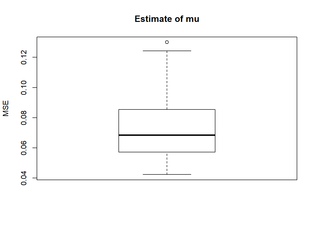

boxplot(result$mse.beta,main='Estimate of beta',ylab='MSE')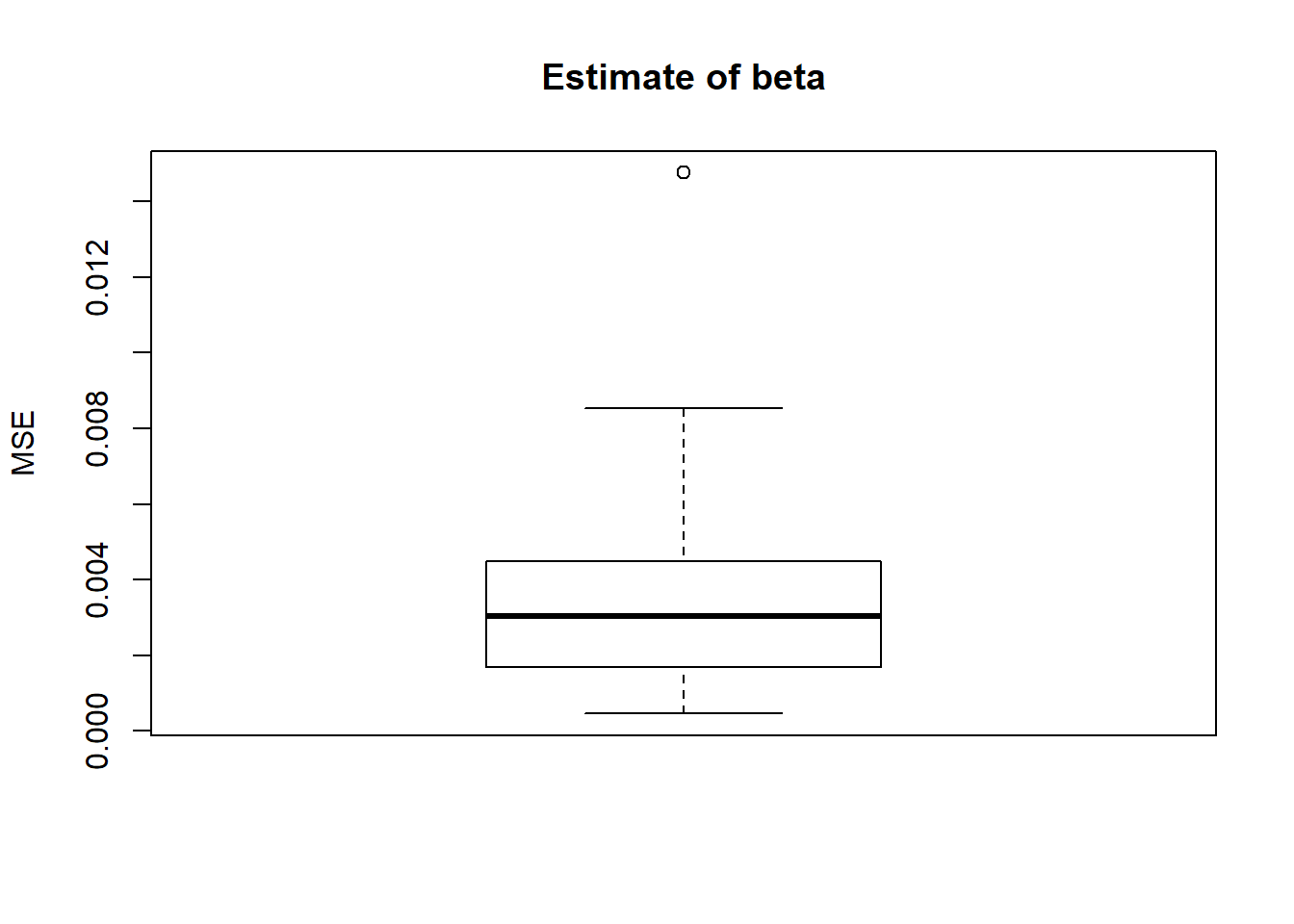

plot(result$y,col='gray80')
lines(mu)
lines(result$mu.hat,col=4)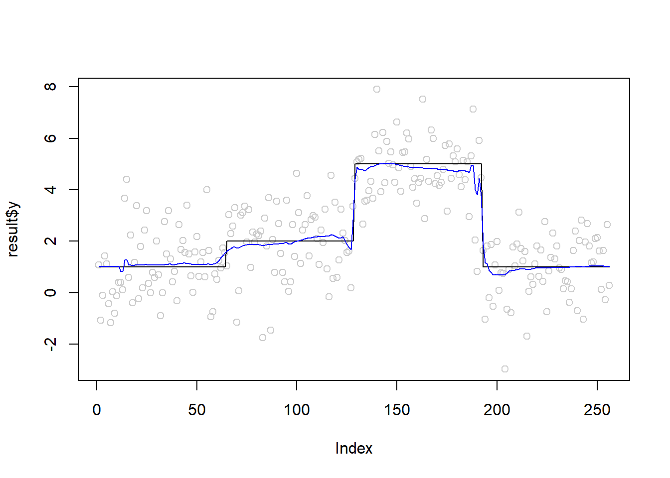

plot(beta,result$beta.hat,xlab = 'True beta', ylab = 'Beta hat')
abline(0,1)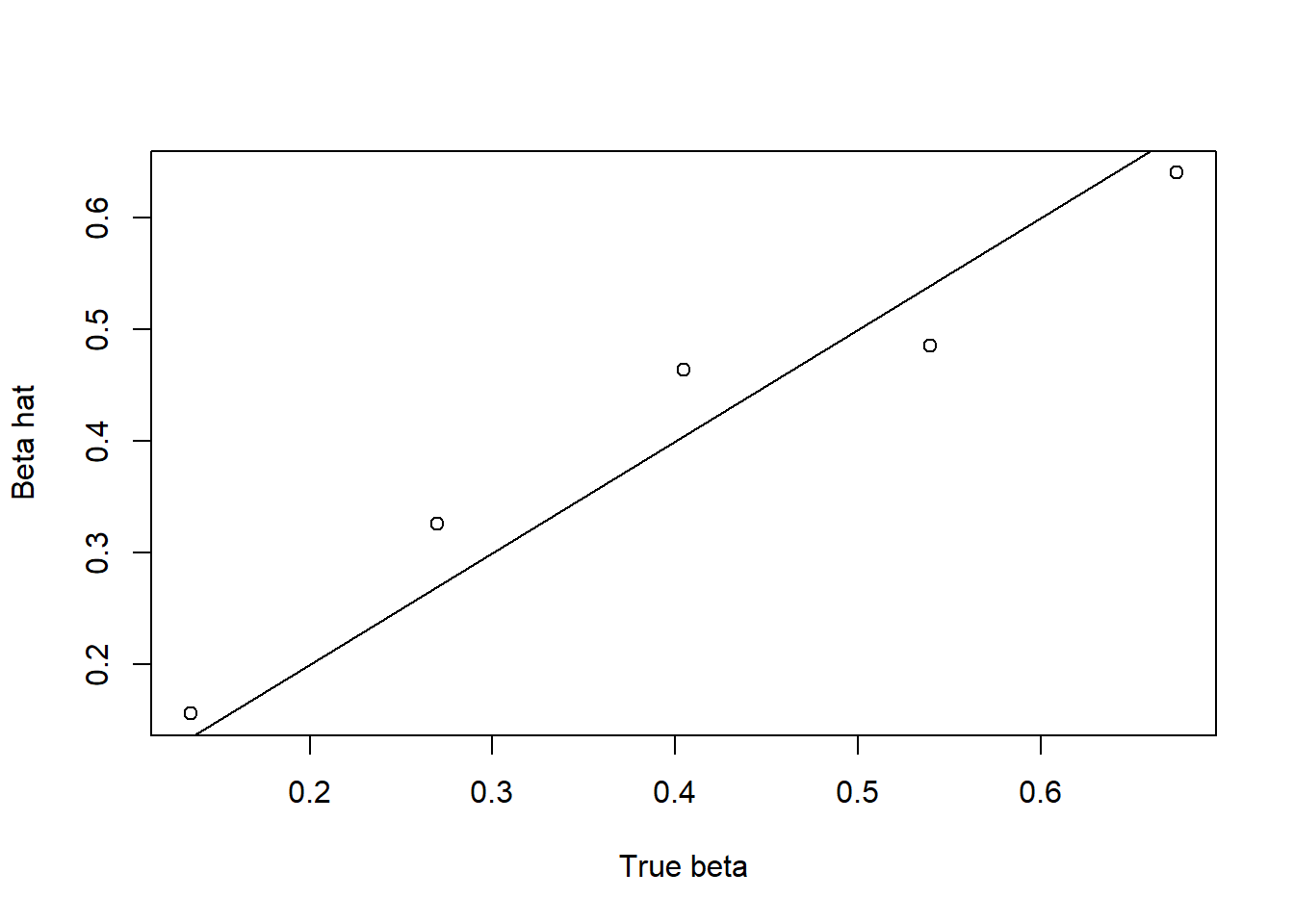

Wave

f=function(x){return(0.5 + 0.2*cos(4*pi*x) + 0.1*cos(24*pi*x))}
mu=f((1:n)/n)

result=simu_study_x(mu,beta,filter.number = 8,family='DaubLeAsymm')
boxplot(result$mse.mu,main='Estimate of mu',ylab='MSE')

boxplot(result$mse.beta,main='Estimate of beta',ylab='MSE')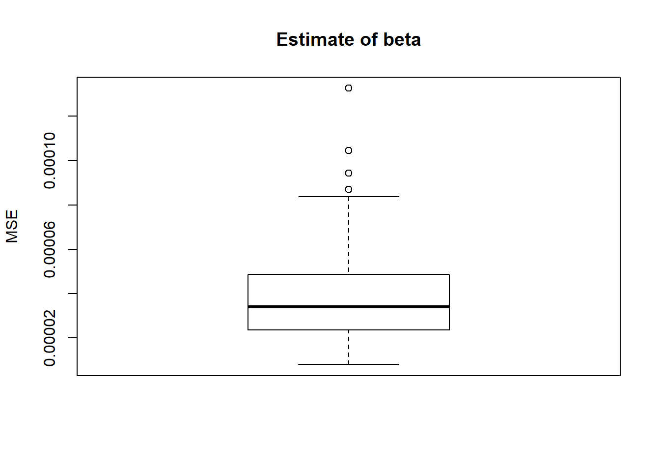

plot(result$y,col='gray80')
lines(mu)
lines(result$mu.hat,col=4)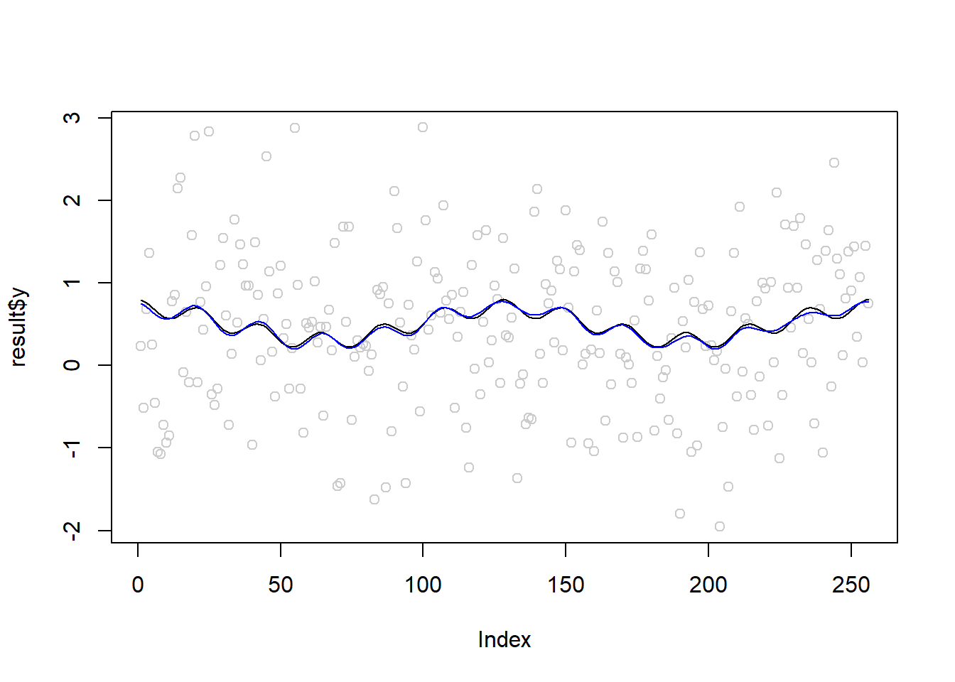

plot(beta,result$beta.hat,xlab = 'True beta', ylab = 'Beta hat')
abline(0,1)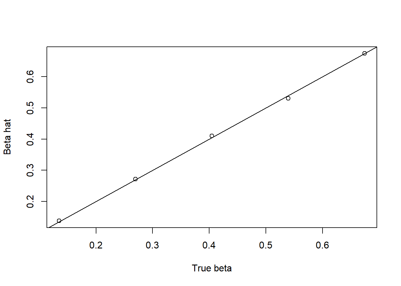

Parabola

r=function(x,c){return((x-c)^2*(x>c)*(x<=1))}
f=function(x){return(0.8 − 30*r(x,0.1) + 60*r(x, 0.2) − 30*r(x, 0.3) +
500*r(x, 0.35) − 1000*r(x, 0.37) + 1000*r(x, 0.41) − 500*r(x, 0.43) +
7.5*r(x, 0.5) − 15*r(x, 0.7) + 7.5*r(x, 0.9))}
mu=f(1:n/n)

result=simu_study_x(mu,beta,filter.number = 8,family='DaubLeAsymm')
boxplot(result$mse.mu,main='Estimate of mu',ylab='MSE')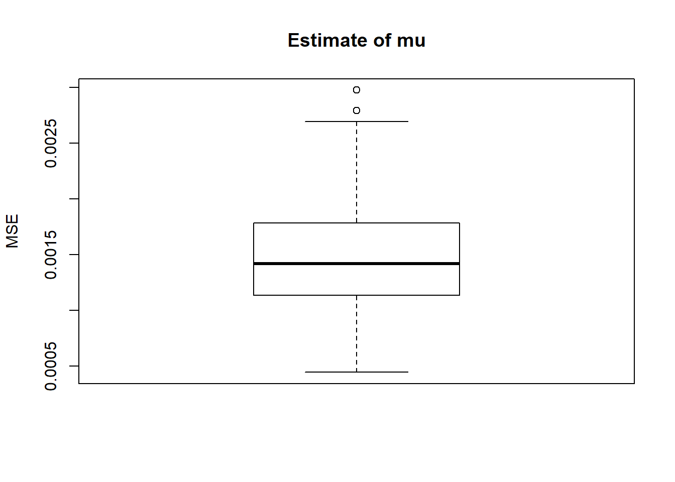

boxplot(result$mse.beta,main='Estimate of beta',ylab='MSE')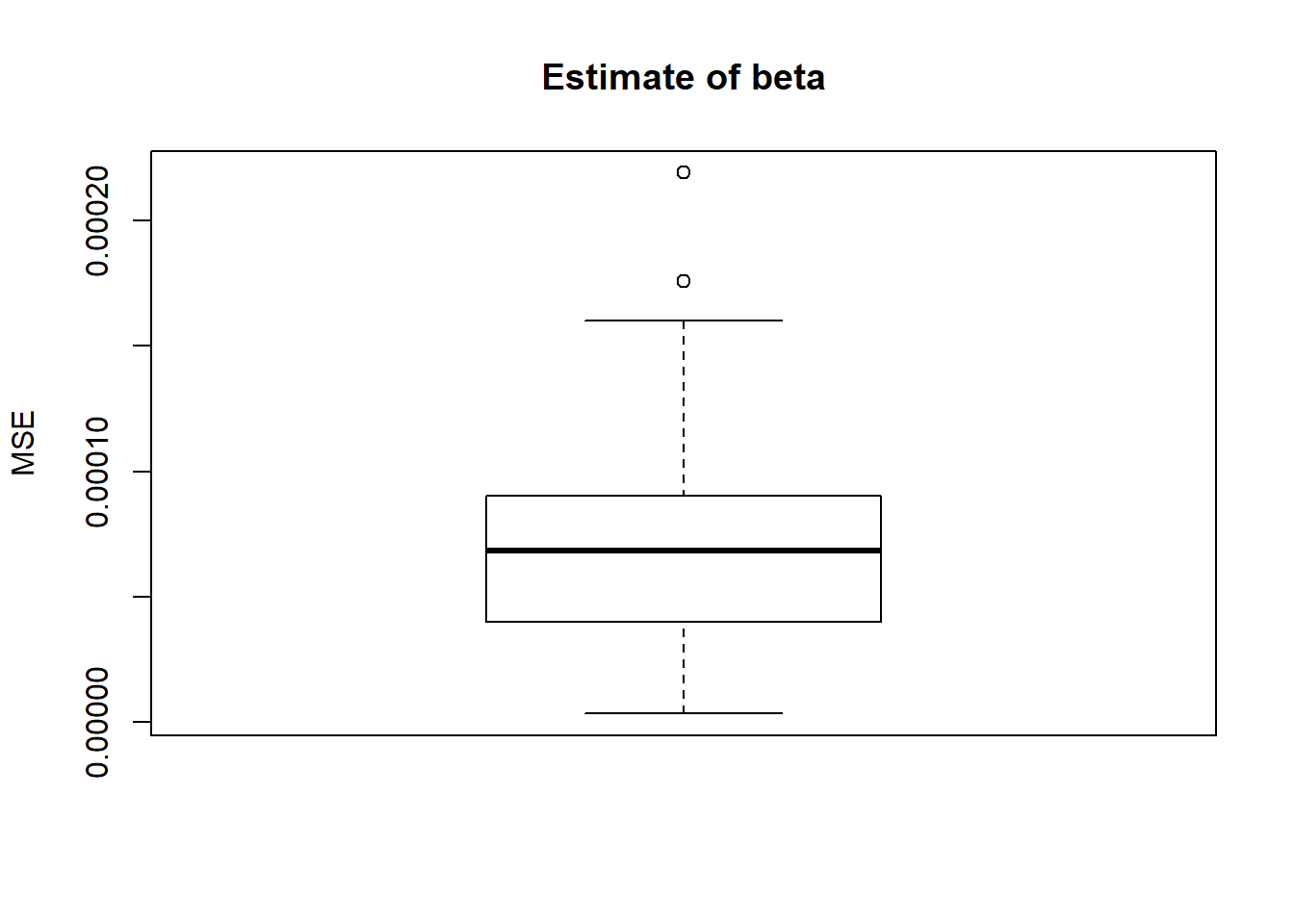

plot(result$y,col='gray80')
lines(mu)
lines(result$mu.hat,col=4)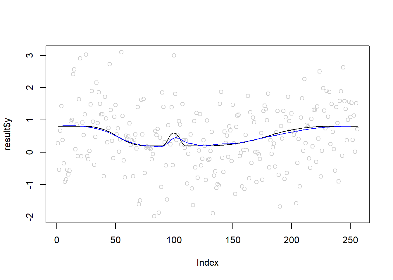

plot(beta,result$beta.hat,xlab = 'True beta', ylab = 'Beta hat')
abline(0,1)

Session information

sessionInfo()

R version 3.4.0 (2017-04-21)
Platform: x86_64-w64-mingw32/x64 (64-bit)
Running under: Windows 10 x64 (build 16299)

Matrix products: default

locale:
[1] LC_COLLATE=English_United States.1252 
[2] LC_CTYPE=English_United States.1252   
[3] LC_MONETARY=English_United States.1252
[4] LC_NUMERIC=C                          
[5] LC_TIME=English_United States.1252    

attached base packages:
[1] stats     graphics  grDevices utils     datasets  methods   base     

other attached packages:
[1] ggplot2_2.2.1    smashrgen_0.1.0  wavethresh_4.6.8 MASS_7.3-47     
[5] caTools_1.17.1   ashr_2.2-7       smashr_1.1-5    

loaded via a namespace (and not attached):
 [1] Rcpp_0.12.16        plyr_1.8.4          compiler_3.4.0     
 [4] git2r_0.21.0        workflowr_1.0.1     R.methodsS3_1.7.1  
 [7] R.utils_2.6.0       bitops_1.0-6        iterators_1.0.8    
[10] tools_3.4.0         digest_0.6.13       tibble_1.3.3       
[13] evaluate_0.10       gtable_0.2.0        lattice_0.20-35    
[16] rlang_0.1.2         Matrix_1.2-9        foreach_1.4.3      
[19] yaml_2.1.19         parallel_3.4.0      stringr_1.3.0      
[22] knitr_1.20          REBayes_1.3         rprojroot_1.3-2    
[25] grid_3.4.0          data.table_1.10.4-3 rmarkdown_1.8      
[28] magrittr_1.5        whisker_0.3-2       backports_1.0.5    
[31] scales_0.4.1        codetools_0.2-15    htmltools_0.3.5    
[34] assertthat_0.2.0    colorspace_1.3-2    stringi_1.1.6      
[37] Rmosek_8.0.69       lazyeval_0.2.1      munsell_0.4.3      
[40] doParallel_1.0.11   pscl_1.4.9          truncnorm_1.0-7    
[43] SQUAREM_2017.10-1   R.oo_1.21.0

This reproducible R Markdown analysis was created with workflowr 1.0.1

Smoothing with covariate

Dongyue Xie

May 24, 2018