Missing data
Dongyue Xie
May 31, 2018
Last updated: 2018-06-03
workflowr checks: (Click a bullet for more information)-
✔ R Markdown file: up-to-date
Great! Since the R Markdown file has been committed to the Git repository, you know the exact version of the code that produced these results.
-
✔ Environment: empty
Great job! The global environment was empty. Objects defined in the global environment can affect the analysis in your R Markdown file in unknown ways. For reproduciblity it’s best to always run the code in an empty environment.
-
✔ Seed:
set.seed(20180501)The command
set.seed(20180501)was run prior to running the code in the R Markdown file. Setting a seed ensures that any results that rely on randomness, e.g. subsampling or permutations, are reproducible. -
✔ Session information: recorded
Great job! Recording the operating system, R version, and package versions is critical for reproducibility.
-
Great! You are using Git for version control. Tracking code development and connecting the code version to the results is critical for reproducibility. The version displayed above was the version of the Git repository at the time these results were generated.✔ Repository version: 09118ad
Note that you need to be careful to ensure that all relevant files for the analysis have been committed to Git prior to generating the results (you can usewflow_publishorwflow_git_commit). workflowr only checks the R Markdown file, but you know if there are other scripts or data files that it depends on. Below is the status of the Git repository when the results were generated:
Note that any generated files, e.g. HTML, png, CSS, etc., are not included in this status report because it is ok for generated content to have uncommitted changes.Ignored files: Ignored: .Rhistory Ignored: .Rproj.user/ Ignored: log/ Untracked files: Untracked: analysis/binom.Rmd Untracked: analysis/glm.Rmd Untracked: analysis/overdis.Rmd Untracked: analysis/smashtutorial.Rmd Untracked: analysis/test.Rmd Untracked: data/treas_bill.csv Untracked: docs/figure/missing.Rmd/ Untracked: docs/figure/smashtutorial.Rmd/ Untracked: docs/figure/test.Rmd/ Unstaged changes: Modified: analysis/ashpmean.Rmd Modified: analysis/nugget.Rmd
Expand here to see past versions:
Treat unevenly spaced data as partly missing data. Set corresponding \(s_t\) to \(10^6\). The missing data are set to 0.
Gaussian
\(Y_t=\mu_t+N(0,s_t^2)\)
library(smashrgen)
spike.f = function(x) (0.75 * exp(-500 * (x - 0.23)^2) + 1.5 * exp(-2000 * (x - 0.33)^2) + 3 * exp(-8000 * (x - 0.47)^2) + 2.25 * exp(-16000 *
    (x - 0.69)^2) + 0.5 * exp(-32000 * (x - 0.83)^2))
n = 256
t = 1:n/n
mu = spike.f(t)+1
rsnr=2
var2 = (1e-04 + 4 * (exp(-550 * (t - 0.2)^2) + exp(-200 * (t - 0.5)^2) + exp(-950 * (t - 0.8)^2)))/1.35
sigma.ini = sqrt(var2)
sigma.t = sigma.ini/mean(sigma.ini) * sd(mu)/rsnr^2
set.seed(12345)
y=mu+rnorm(n,0,sigma.t)

# No missing data fit
fit=smash.gaus(y,sigma=sigma.t)
plot(y,type='p',col='gray80',main='No missing data')
lines(mu)
lines(fit,type='l',col=4)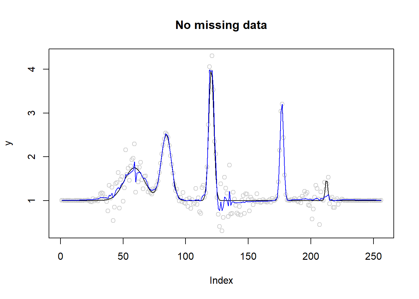
# missing data 1%
idx=sample(1:n,n*0.01)

idx
[1] 87 172y.miss=y
y.miss[idx]=0
sigma.miss=sigma.t
sigma.miss[idx]=10^6
fit=smash.gaus(y.miss,sigma=sigma.miss)
plot(y.miss,type='p',col='gray80',main='Missing 1% data')
lines(fit,col=4)
lines(idx,fit[idx],type='p',pch=16,col=2)
lines(mu,type='l')
legend('topright',c('smash.gaus','Missing points','True mu'),col=c(4,2,1),pch=c(NA,16,NA),lty=c(1,NA,1))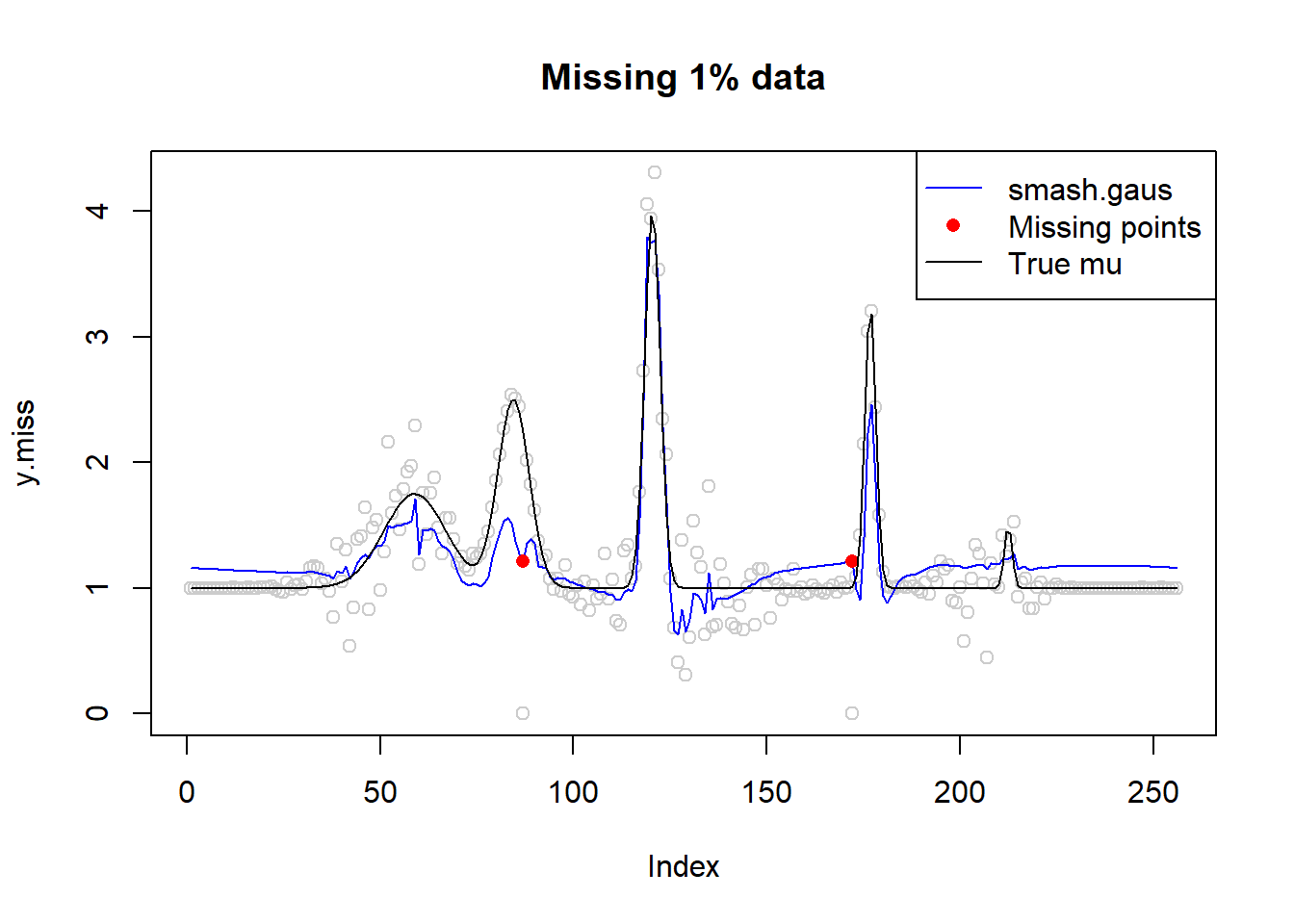
# # pretend variance are unknown
# fit2=smash.gaus(y.miss)
# plot(fit2,type='l',col=4,ylim=c(-0.5,3),main='Missing 1% data, variance unknown')
# lines(mu)

# missing data 5%
idx=sample(1:n,n*0.05)

sort(idx)
[1] 32 49 55 63 74 83 109 148 175 191 198 223y.miss=y
y.miss[idx]=0
sigma.miss=sigma.t
sigma.miss[idx]=10^6
fit=smash.gaus(y.miss,sigma=sigma.miss)
plot(y.miss,type='p',col='gray80',main='Missing 5% data')
lines(fit,col=4)
lines(idx,fit[idx],type='p',pch=16,col=2)
lines(mu,type='l')
legend('topright',c('smash.gaus','Missing points','True mu'),col=c(4,2,1),pch=c(NA,16,NA),lty=c(1,NA,1))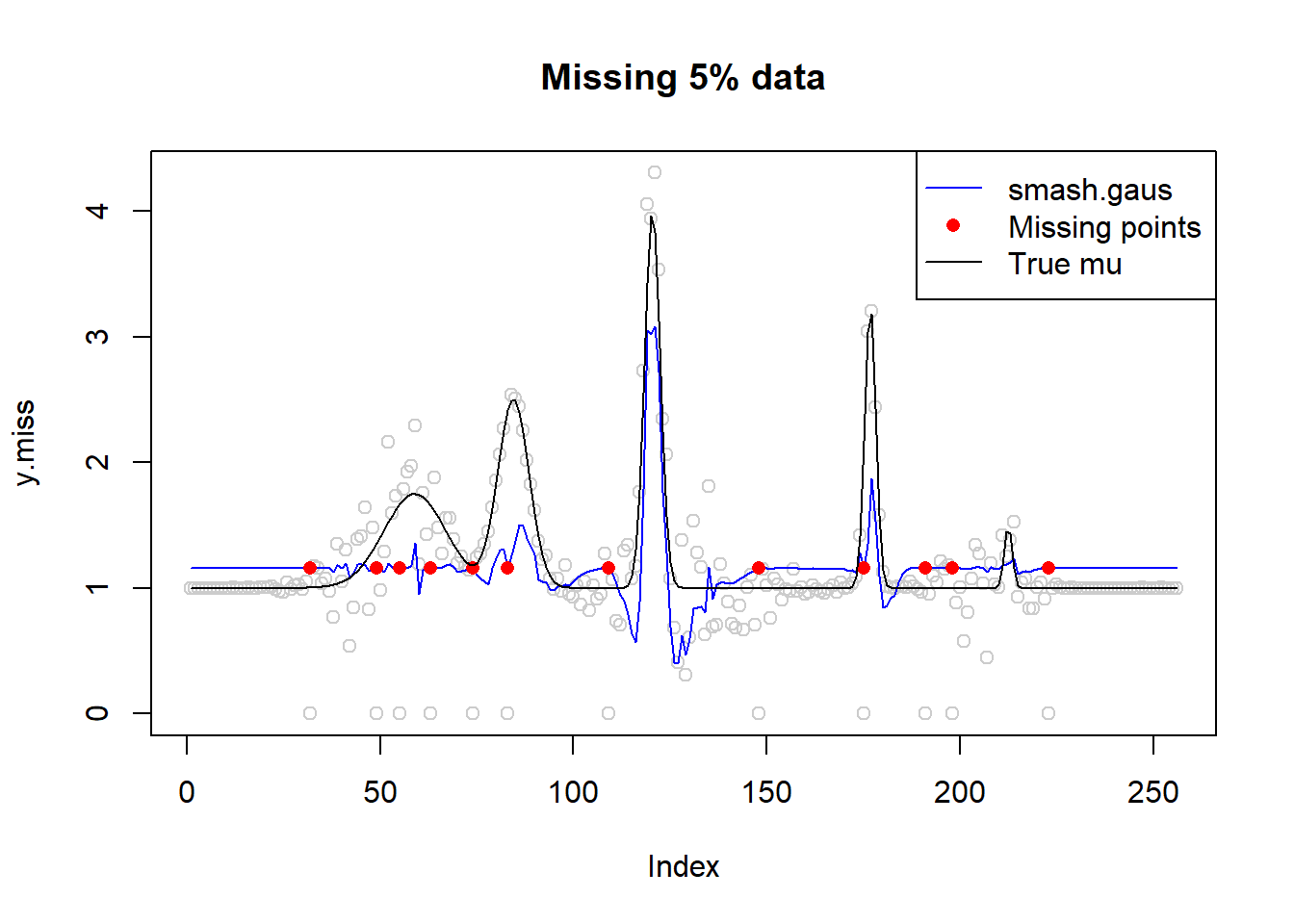
# # pretend variance are unknown
# fit2=smash.gaus(y.miss)
# plot(fit2,type='l',col=4,ylim=c(-0.5,3),main='Missing 5% data, variance unknown')
# lines(mu)

# missing data 10%
idx=sample(1:n,n*0.1)

sort(idx)
[1] 5 30 58 62 64 78 90 99 110 128 129 130 142 147 163 170 171
[18] 179 203 204 205 225 237 255 256y.miss=y
y.miss[idx]=0
sigma.miss=sigma.t
sigma.miss[idx]=10^6
fit=smash.gaus(y.miss,sigma=sigma.miss)
plot(y.miss,type='p',col='gray80',main='Missing 10% data')
lines(fit,col=4)
lines(idx,fit[idx],type='p',pch=16,col=2)
lines(mu,type='l')
legend('topright',c('smash.gaus','Missing points','True mu'),col=c(4,2,1),pch=c(NA,16,NA),lty=c(1,NA,1))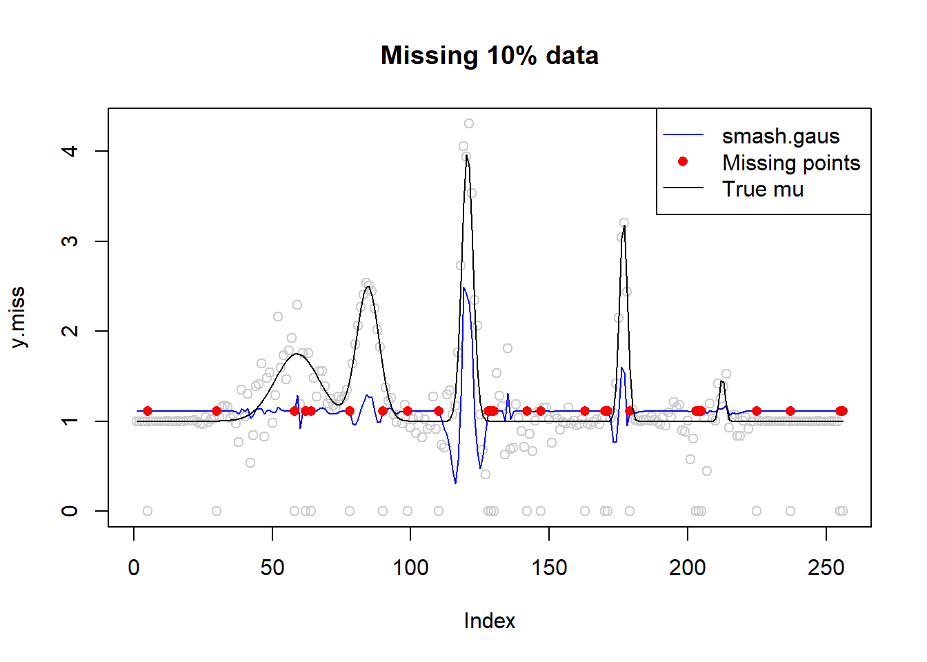
# missing data 20%
idx=sample(1:n,n*0.2)

sort(idx)
[1] 3 4 12 17 22 25 36 43 47 53 54 57 59 65 76 89 95
[18] 96 109 114 119 125 128 130 139 142 145 148 152 155 159 163 167 170
[35] 176 178 193 205 212 221 227 228 230 234 239 240 243 244 247 252 254y.miss=y
y.miss[idx]=0
sigma.miss=sigma.t
sigma.miss[idx]=10^6
fit=smash.gaus(y.miss,sigma=sigma.miss)
plot(y.miss,type='p',col='gray80',main='Missing 20% data')
lines(fit,col=4)
lines(idx,fit[idx],type='p',pch=16,col=2)
lines(mu,type='l')
legend('topright',c('smash.gaus','Missing points','True mu'),col=c(4,2,1),pch=c(NA,16,NA),lty=c(1,NA,1))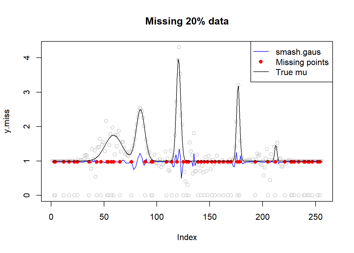
Why it’s not working?
\(y=\mu+\epsilon\)
\(Wy=W\mu+W\epsilon \Rightarrow\tilde y=\tilde\mu+N(0,diag(\tilde\sigma^2))\)
We are shrinking the wavelet coefficients(\(\tilde\mu\)) not \(y\)! If we set the missing data’s \(s_t\) very large, then all the variance of corresponding wavelet coefficients that involve missing data are very large. Thus, a large number of wavelet coefficients(essentially differences) are shrinked to zero, including those should not be done so.
An simple example:
mu=c(1,1,1,1,4,4,4,4)
y=mu+rnorm(8,0,0.8)
sigma=rep(0.8,8)

w=t(GenW(filter.number = 1,family='DaubExPhase'))

y.miss=y
y.miss[6]=0
sigma.miss=sigma
sigma.miss[6]=1e6
y.tilde=w%*%y.miss
sigma.tilde=w%*%diag(sigma.miss)%*%t(w)
y.ash=ash(as.numeric(y.tilde),as.numeric(diag(sigma.tilde)))$result$PosteriorMean
y.hat=t(w)%*%y.ash
plot(wd(y.miss,filter.number = 1,family='DaubExPhase'),main = 'Decomposition of Y with missing data set to 0')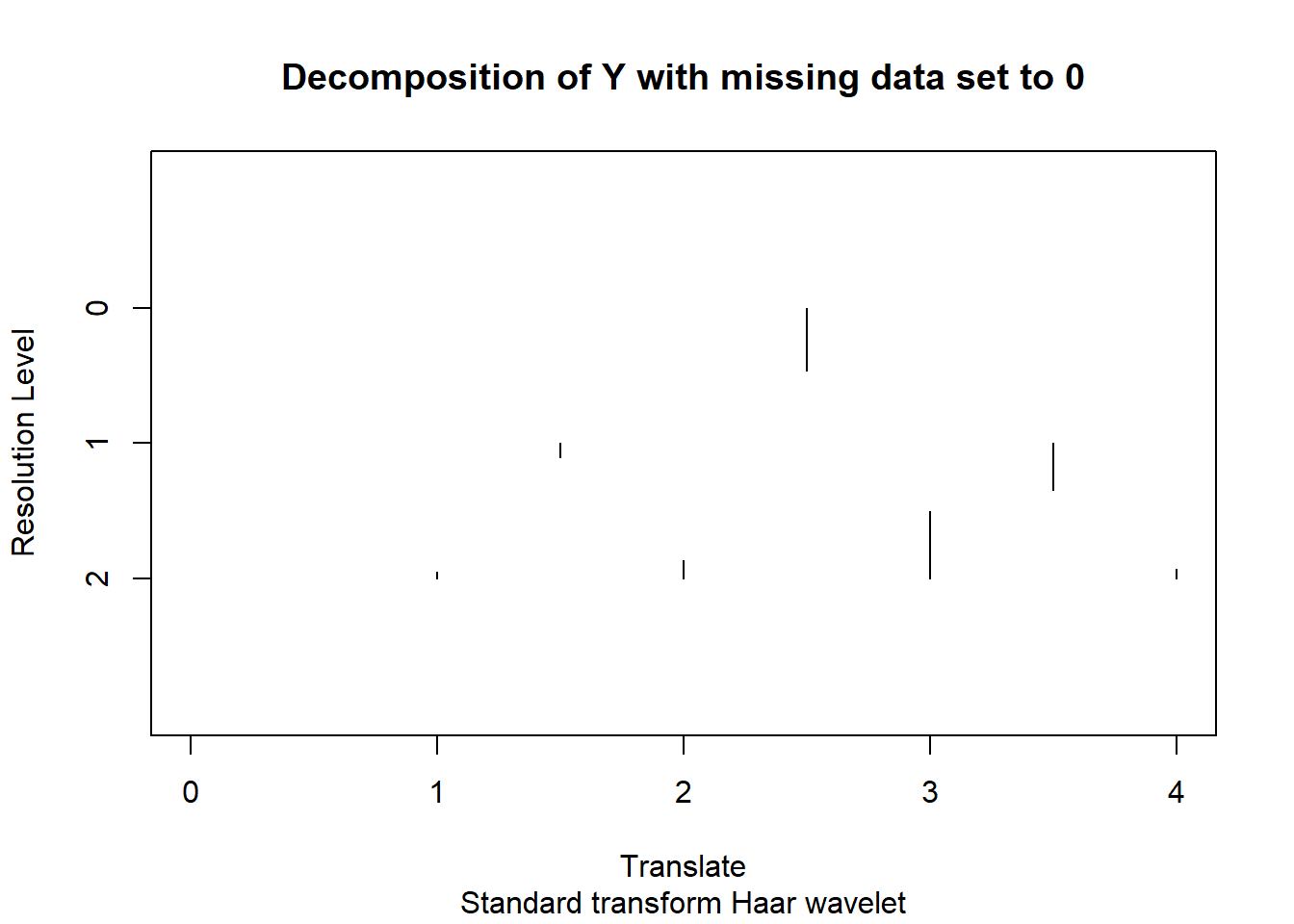
[1] 2.850042 2.850042 2.850042plot(wd(y,filter.number = 1,family='DaubExPhase'),main='Decomposition of Y, no missing data')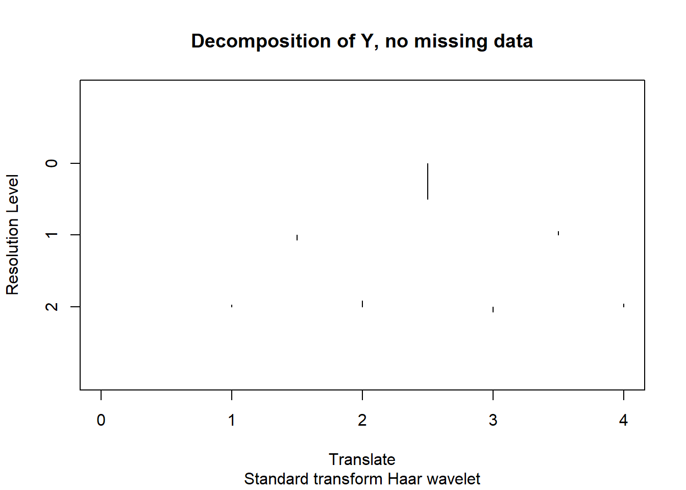
[1] 4.411388 4.411388 4.411388Let’s look at \(\tilde\sigma\):
diag(sigma.tilde)[1] 125000.7 0.8 0.8 500000.4 0.8 0.8 250000.6 125000.7The 2nd-5th ones are from level 2, 6th-7th are from level 1 and the last one corresponds to level 0.
From the plot of coefficients, what we really want to set to 0 is 4th and 7th. But the 8th one also has huge variance.
Can we manually choose what levels to shrink using large variance?
I don’t think it’s practical, especially when the length of sequence and number of missing data are large. Maybe the only criterion is whether it’s visually appealing.
Session information
sessionInfo()R version 3.4.0 (2017-04-21)
Platform: x86_64-w64-mingw32/x64 (64-bit)
Running under: Windows 10 x64 (build 16299)
Matrix products: default
locale:
[1] LC_COLLATE=English_United States.1252
[2] LC_CTYPE=English_United States.1252
[3] LC_MONETARY=English_United States.1252
[4] LC_NUMERIC=C
[5] LC_TIME=English_United States.1252
attached base packages:
[1] stats graphics grDevices utils datasets methods base
other attached packages:
[1] smashrgen_0.1.0 wavethresh_4.6.8 MASS_7.3-47 caTools_1.17.1
[5] ashr_2.2-7 smashr_1.1-5
loaded via a namespace (and not attached):
[1] Rcpp_0.12.16 compiler_3.4.0 git2r_0.21.0
[4] workflowr_1.0.1 R.methodsS3_1.7.1 R.utils_2.6.0
[7] bitops_1.0-6 iterators_1.0.8 tools_3.4.0
[10] digest_0.6.13 evaluate_0.10 lattice_0.20-35
[13] Matrix_1.2-9 foreach_1.4.3 yaml_2.1.19
[16] parallel_3.4.0 stringr_1.3.0 knitr_1.20
[19] REBayes_1.3 rprojroot_1.3-2 grid_3.4.0
[22] data.table_1.10.4-3 rmarkdown_1.8 magrittr_1.5
[25] whisker_0.3-2 backports_1.0.5 codetools_0.2-15
[28] htmltools_0.3.5 assertthat_0.2.0 stringi_1.1.6
[31] Rmosek_8.0.69 doParallel_1.0.11 pscl_1.4.9
[34] truncnorm_1.0-7 SQUAREM_2017.10-1 R.oo_1.21.0 This reproducible R Markdown analysis was created with workflowr 1.0.1