Shrink R squared - examples
Dongyue Xie
2019-01-21
Last updated: 2020-09-07
Checks: 7 0
Knit directory: smash-gen/
This reproducible R Markdown analysis was created with workflowr (version 1.5.0). The Checks tab describes the reproducibility checks that were applied when the results were created. The Past versions tab lists the development history.
Great! Since the R Markdown file has been committed to the Git repository, you know the exact version of the code that produced these results.
Great job! The global environment was empty. Objects defined in the global environment can affect the analysis in your R Markdown file in unknown ways. For reproduciblity it’s best to always run the code in an empty environment.
The command set.seed(20180501) was run prior to running the code in the R Markdown file. Setting a seed ensures that any results that rely on randomness, e.g. subsampling or permutations, are reproducible.
Great job! Recording the operating system, R version, and package versions is critical for reproducibility.
Nice! There were no cached chunks for this analysis, so you can be confident that you successfully produced the results during this run.
Great job! Using relative paths to the files within your workflowr project makes it easier to run your code on other machines.
Great! You are using Git for version control. Tracking code development and connecting the code version to the results is critical for reproducibility. The version displayed above was the version of the Git repository at the time these results were generated.
Note that you need to be careful to ensure that all relevant files for the analysis have been committed to Git prior to generating the results (you can use wflow_publish or wflow_git_commit). workflowr only checks the R Markdown file, but you know if there are other scripts or data files that it depends on. Below is the status of the Git repository when the results were generated:
Ignored files:
    Ignored:    .DS_Store
    Ignored:    .Rhistory
    Ignored:    .Rproj.user/
    Ignored:    analysis/figure/
    Ignored:    data/.DS_Store

Untracked files:
    Untracked:  analysis/chipexoeg.Rmd
    Untracked:  analysis/efsd.Rmd
    Untracked:  analysis/pln_smooth.Rmd
    Untracked:  analysis/pre0221.Rmd
    Untracked:  analysis/smashadditive.Rmd
    Untracked:  analysis/talk1011.Rmd
    Untracked:  data/chipexo_examples/
    Untracked:  data/chipseq_examples/
    Untracked:  talk.Rmd
    Untracked:  talk.html
    Untracked:  talk.pdf

Unstaged changes:
    Modified:   analysis/binomial.Rmd
    Modified:   analysis/fda.Rmd
    Modified:   analysis/protein.Rmd
    Modified:   analysis/r2.Rmd
    Modified:   analysis/sigma.Rmd
Note that any generated files, e.g. HTML, png, CSS, etc., are not included in this status report because it is ok for generated content to have uncommitted changes.
These are the previous versions of the R Markdown and HTML files. If you’ve configured a remote Git repository (see ?wflow_git_remote), click on the hyperlinks in the table below to view them.
| File | Version | Author | Date | Message |
|---|---|---|---|---|
| Rmd | e723bec | Dongyue Xie | 2020-09-07 | wflow_publish(“analysis/r2b.Rmd”) |
| html | 5a3ca6f | Dongyue Xie | 2019-02-10 | Build site. |
| Rmd | 63863c7 | Dongyue Xie | 2019-02-10 | wflow_publish(“analysis/r2b.Rmd”) |
| html | e49cf2f | Dongyue Xie | 2019-02-10 | Build site. |
| Rmd | d255e06 | Dongyue Xie | 2019-02-10 | wflow_publish(“analysis/r2b.Rmd”) |
| html | c6f9a91 | Dongyue Xie | 2019-02-10 | Build site. |
| Rmd | 7e08c59 | Dongyue Xie | 2019-02-10 | wflow_publish(“analysis/r2b.Rmd”) |
| html | c7f4704 | Dongyue Xie | 2019-01-27 | Build site. |
| Rmd | a1a64c5 | Dongyue Xie | 2019-01-27 | wflow_publish(“analysis/r2b.Rmd”) |
| html | 9ce257c | Dongyue Xie | 2019-01-27 | Build site. |
| Rmd | d6bcb1a | Dongyue Xie | 2019-01-27 | wflow_publish(“analysis/r2b.Rmd”) |
| html | 97b73fc | Dongyue Xie | 2019-01-22 | Build site. |
| Rmd | b5029e2 | Dongyue Xie | 2019-01-22 | wflow_publish(“analysis/r2b.Rmd”) |
| html | ad12c40 | Dongyue Xie | 2019-01-22 | Build site. |
| Rmd | 11f83fb | Dongyue Xie | 2019-01-22 | wflow_publish(“analysis/r2b.Rmd”) |
For the method used in these examples, see here
True \(R^2\) is defined as \(R^2=\frac{var(X\beta)}{var(y)}=\frac{var(y)-\sigma^2}{var(y)}=1-\frac{\sigma^2}{var(y)}=1-\frac{\sigma^2}{\sigma^2+var(X\beta)}\)
Ajusted R^2: \(1-\frac{\sum(y_i-\hat y_i)^2/(n-p-1)}{\sum(y_i-\bar y)^2/(n-1)}\)
Shrunk adjusted R^2: use
fashshrinking \(fash.output=\log(\frac{\sum(y_i-\hat y_i)^2/(n-p-1)}{\sum(y_i-\bar y)^2/(n-1)})\) then shrunk adjusted R^2 is \(1-\exp(fash.output)\)Shrunk R^2: use
fashshrinking \(fash.output=\log(\frac{\sum(y_i-\hat y_i)^2/(n-1)}{\sum(y_i-\bar y)^2/(n-1)})\) then shrunk adjusted R^2 is \(1-\exp(fash.output)\)Another Shrunk R^2: shrink all \(\betas\) using
ash, obtain posterior means then calculate \(\hat\sigma^2\) then obtain \(\frac{var(X\hat\beta)}{var(\hat\beta)+\hat\sigma^2}\).
(note: this is the old idea which introduces bias to R^2 when multiplying \(\frac{n-p-1}{n-1}\) so I discard this method.)(Shrunk R^2 = \(1 - \exp(fash.output)*\frac{n-p-1}{n-1}\), because \(R^2=1-\frac{\sum(y_i-\hat y_i)^2}{\sum(y_i-\bar y)^2}=1-\frac{\sum(y_i-\hat y_i)^2/(n-p-1)}{\sum(y_i-\bar y)^2/(n-1)}*\frac{n-p-1}{n-1}=1-(1-adjR^2)*\frac{n-p-1}{n-1}\))
R Function
R function for shrinking adjusted R/ R squared:
library(ashr)
#'@param R2: R squared from linear regression model fit
#'@param n: sample size
#'@param p: the number of covariates
#'@output shrunk R squared.

ash_ar2=function(R2,n,p){
  df1=n-p-1
  df2=n-1
  log.ratio=log((1-R2)/(df1)*(df2))
  shrink.log.ratio=ash(log.ratio,1,lik=lik_logF(df1=df1,df2=df2))$result$PosteriorMean
  ar2=1-exp(shrink.log.ratio)
  return(ar2)
}


# ash_r2=function(R2,n,p){
#   df1=n-1
#   df2=n-1
#   log.ratio=log(1-R2)
#   shrink.log.ratio=ash(log.ratio,1,lik=lik_logF(df1=df1,df2=df2))$result$PosteriorMean
#   r2=1-exp(shrink.log.ratio)
#   return(r2)
# }

ash_r2=function(R2,n,p){
  df1=p
  df2=n-p-1
  log.ratio=log(R2/(1-R2)/df1*df2)
  shrink.log.ratio=ash(log.ratio,1,lik=lik_logF(df1=df1,df2=df2),
                       mixcompdist="+uniform")$result$PosteriorMean
  #r2=(exp(shrink.log.ratio)-1)/(n/p+1)
  r2=(exp(shrink.log.ratio)-1)
  r2/(1+r2)
}
Compare Shrunk \(R^2\) with True \(R2\).
Assume linear model \(y=X\beta+\epsilon\) where \(\epsilon\sim N(0,\sigma^2I)\)
- n=100, p=5. Each cordinate of \(\beta\) ranges from 0 to 1, for example \(\beta=(0,0,0,0,0)\),…,\(\beta=(0.1,0.1,0.1,0.1,0.1)\),…, \(\beta=(1,1,1,1,1)\) etc.
If I generate X from Uniform(0,1), then fash shirnks all \(R^2\) to 0. If generate X from Uniform(0,2), then it does not
X from Uniform(0,1):
set.seed(1234)

n=100
p=5
R2=c()
R2a=c()
trueR2=c()

beta.list=seq(0,1,length.out = 100)
X=matrix(runif(n*(p),0,1),n,p)
for (i in 1:length(beta.list)) {

  beta=rep(beta.list[i],p)
  y=X%*%beta+rnorm(n)
  datax=data.frame(X=X,y=y)
  mod=lm(y~.,datax)
  mod.sy=summary(mod)
  R2[i]=mod.sy$r.squared
  R2a[i]=mod.sy$adj.r.squared
  trueR2[i]=var(X%*%beta)/(1+var(X%*%beta))
}
R2s=ash_r2(R2,n,p)
R2as=ash_ar2(R2,n,p)
plot(beta.list,R2,ylim=range(c(R2,R2a,R2s,R2as,trueR2)),main='',xlab='beta',ylab='',type='l')
lines(beta.list,R2a,col=2)
lines(beta.list,R2as,col=3)
lines(beta.list,R2s,col=4)
lines(beta.list,trueR2,col='grey80')
abline(h=0,lty=2)
legend('topleft',c('R^2','Adjusted R^2','Adjusted R^2 fash','R^2 fash','True R^2'),lty=c(1,1,1,1,1),col=c(1,2,3,4,'grey80'))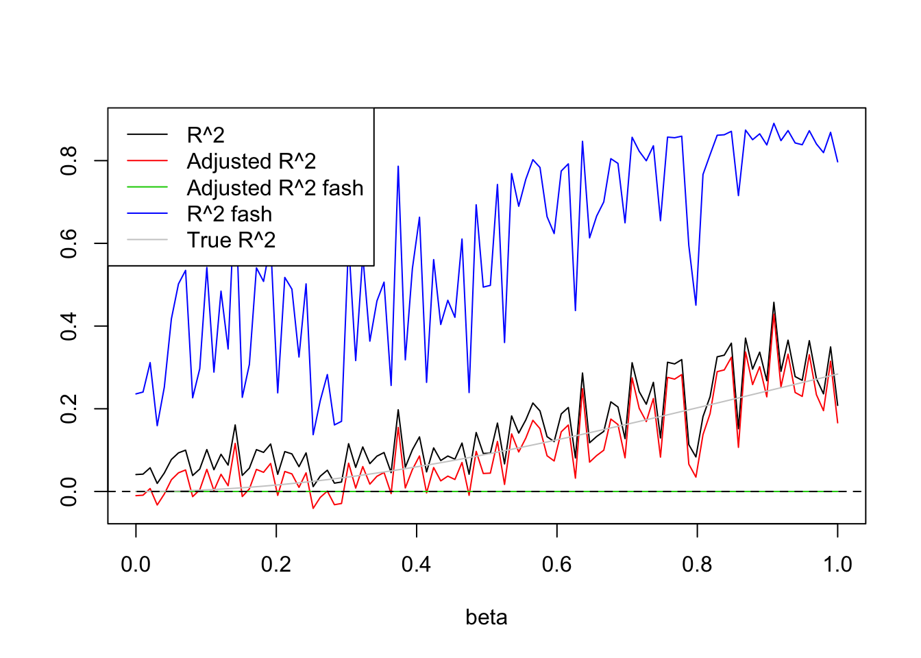
plot(trueR2,R2,type='l',ylim=range(c(R2,R2a,R2s,R2as,trueR2)))
lines(trueR2,R2a,col=2)
lines(trueR2,R2as,col=3)
lines(trueR2,R2s,col=4)
lines(trueR2,trueR2,col='grey80')
legend('topleft',c('R^2','Adjusted R^2','Adjusted R^2 fash','R^2 fash'),lty=c(1,1,1,1),col=c(1,2,3,4))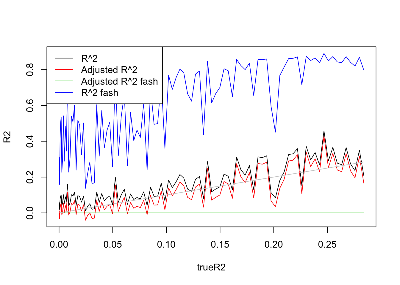
Uniform(0,3):
set.seed(1234)

n=100
p=5
R2=c()
R2a=c()
trueR2=c()

beta.list=seq(0,1,length.out = 100)
X=matrix(runif(n*(p),0,3),n,p)
for (i in 1:length(beta.list)) {

  beta=rep(beta.list[i],p)
  y=X%*%beta+rnorm(n)
  datax=data.frame(X=X,y=y)
  mod=lm(y~.,datax)
  mod.sy=summary(mod)
  R2[i]=mod.sy$r.squared
  R2a[i]=mod.sy$adj.r.squared
  trueR2[i]=var(X%*%beta)/(1+var(X%*%beta))
}
R2s=ash_r2(R2,n,p)
R2as=ash_ar2(R2,n,p)
plot(beta.list,R2,ylim=range(c(R2,R2a,R2s,R2as,trueR2)),main='',xlab='beta',ylab='',type='l')
lines(beta.list,R2a,col=2)
lines(beta.list,R2as,col=3)
lines(beta.list,R2s,col=4)
lines(beta.list,trueR2,col='grey80')
abline(h=0,lty=2)
legend('topleft',c('R^2','Adjusted R^2','Adjusted R^2 fash','R^2 fash','True R^2'),lty=c(1,1,1,1,1),col=c(1,2,3,4,'grey80'))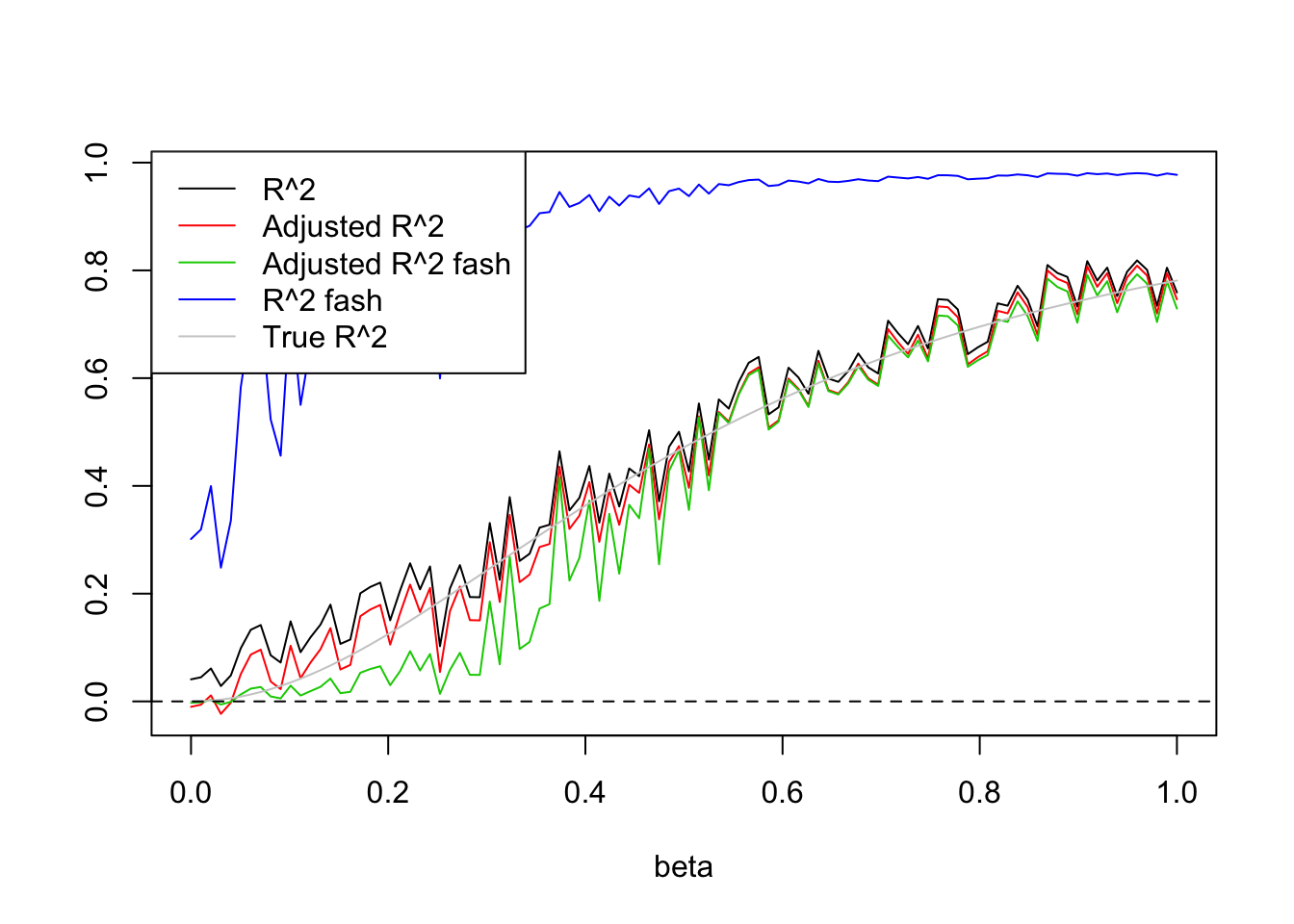
plot(trueR2,R2,type='l',ylim=range(c(R2,R2a,R2s,R2as,trueR2)))
lines(trueR2,R2a,col=2)
lines(trueR2,R2as,col=3)
lines(trueR2,R2s,col=4)
lines(trueR2,trueR2,col='grey80')
legend('topleft',c('R^2','Adjusted R^2','Adjusted R^2 fash','R^2 fash'),lty=c(1,1,1,1),col=c(1,2,3,4))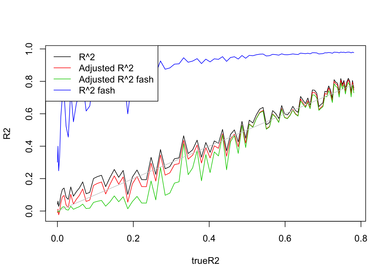
Uniform(0,5):
set.seed(1234)

n=100
p=5
R2=c()
R2a=c()
trueR2=c()

beta.list=seq(0,1,length.out = 100)
X=matrix(runif(n*(p),0,5),n,p)
for (i in 1:length(beta.list)) {

  beta=rep(beta.list[i],p)
  y=X%*%beta+rnorm(n)
  datax=data.frame(X=X,y=y)
  mod=lm(y~.,datax)
  mod.sy=summary(mod)
  R2[i]=mod.sy$r.squared
  R2a[i]=mod.sy$adj.r.squared
  trueR2[i]=var(X%*%beta)/(1+var(X%*%beta))
}
R2s=ash_r2(R2,n,p)
R2as=ash_ar2(R2,n,p)
plot(beta.list,R2,ylim=range(c(R2,R2a,R2s,R2as,trueR2)),main='',xlab='beta',ylab='',type='l')
lines(beta.list,R2a,col=2)
lines(beta.list,R2as,col=3)
lines(beta.list,R2s,col=4)
lines(beta.list,trueR2,col='grey80')
abline(h=0,lty=2)
legend('topleft',c('R^2','Adjusted R^2','Adjusted R^2 fash','R^2 fash','True R^2'),lty=c(1,1,1,1,1),col=c(1,2,3,4,'grey80'))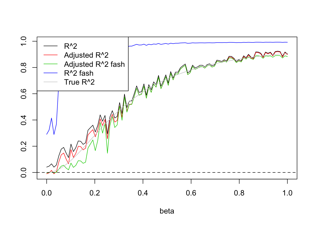
plot(trueR2,R2,type='l',ylim=range(c(R2,R2a,R2s,R2as,trueR2)))
lines(trueR2,R2a,col=2)
lines(trueR2,R2as,col=3)
lines(trueR2,R2s,col=4)
lines(trueR2,trueR2,col='grey80')
legend('topleft',c('R^2','Adjusted R^2','Adjusted R^2 fash','R^2 fash'),lty=c(1,1,1,1),col=c(1,2,3,4))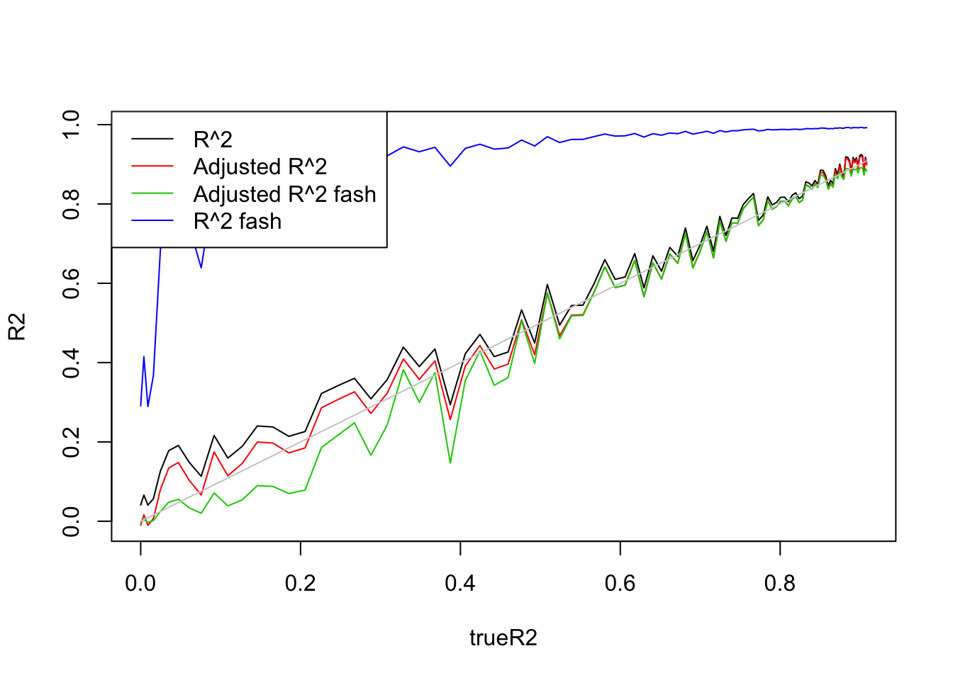
- Increase \(p\) to 20.
This time, if I generate X from Uniform(0,1), then fash does not shirnk all \(R^2\) to 0.
Uniform(0,1):
set.seed(1234)

n=100
p=20
R2=c()
R2a=c()
trueR2=c()

beta.list=seq(0,1,length.out = 100)
X=matrix(runif(n*(p),0,1),n,p)
for (i in 1:length(beta.list)) {

  beta=rep(beta.list[i],p)
  y=X%*%beta+rnorm(n)
  datax=data.frame(X=X,y=y)
  mod=lm(y~.,datax)
  mod.sy=summary(mod)
  R2[i]=mod.sy$r.squared
  R2a[i]=mod.sy$adj.r.squared
  trueR2[i]=var(X%*%beta)/(1+var(X%*%beta))
}
R2s=ash_r2(R2,n,p)
R2as=ash_ar2(R2,n,p)
plot(beta.list,R2,ylim=range(c(R2,R2a,R2s,R2as,trueR2)),main='',xlab='beta',ylab='',type='l')
lines(beta.list,R2a,col=2)
lines(beta.list,R2as,col=3)
lines(beta.list,R2s,col=4)
lines(beta.list,trueR2,col='grey80')
abline(h=0,lty=2)
legend('topleft',c('R^2','Adjusted R^2','Adjusted R^2 fash','R^2 fash','True R^2'),lty=c(1,1,1,1,1),col=c(1,2,3,4,'grey80'))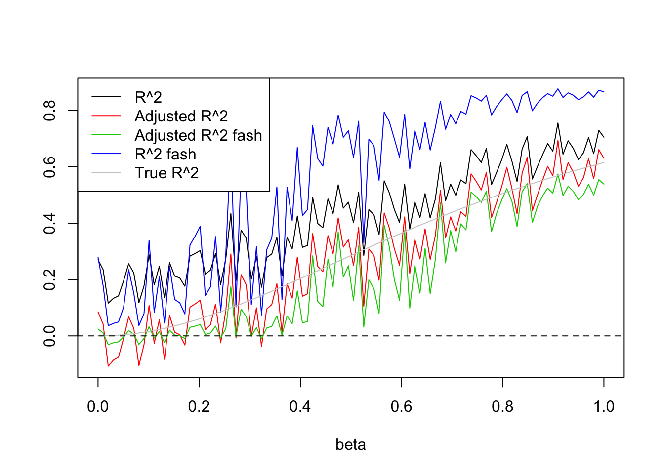
plot(trueR2,R2,type='l',ylim=range(c(R2,R2a,R2s,R2as,trueR2)))
lines(trueR2,R2a,col=2)
lines(trueR2,R2as,col=3)
lines(trueR2,R2s,col=4)
lines(trueR2,trueR2,col='grey80')
legend('topleft',c('R^2','Adjusted R^2','Adjusted R^2 fash','R^2 fash'),lty=c(1,1,1,1),col=c(1,2,3,4))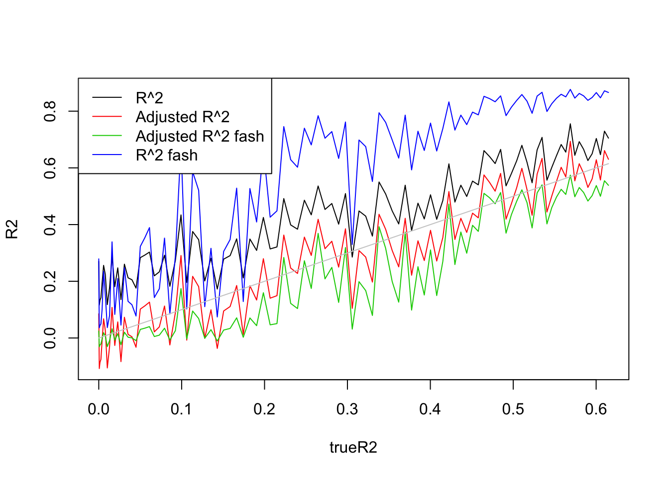
- \(n=30, p=3\).
This time, I have to generate X from at least Uniform(0,3) to avoid over-shrinkage of fash. Here, I tried Uniform(0,5)
Uniform(0,5):
set.seed(1234)

n=30
p=3
R2=c()
R2a=c()
trueR2=c()

beta.list=seq(0,1,length.out = 100)
X=matrix(runif(n*(p),0,5),n,p)
for (i in 1:length(beta.list)) {

  beta=rep(beta.list[i],p)
  y=X%*%beta+rnorm(n)
  datax=data.frame(X=X,y=y)
  mod=lm(y~.,datax)
  mod.sy=summary(mod)
  R2[i]=mod.sy$r.squared
  R2a[i]=mod.sy$adj.r.squared
  trueR2[i]=var(X%*%beta)/(1+var(X%*%beta))
}
R2s=ash_r2(R2,n,p)
R2as=ash_ar2(R2,n,p)
plot(beta.list,R2,ylim=range(c(R2,R2a,R2s,R2as,trueR2)),main='',xlab='beta',ylab='',type='l')
lines(beta.list,R2a,col=2)
lines(beta.list,R2as,col=3)
lines(beta.list,R2s,col=4)
lines(beta.list,trueR2,col='grey80')
abline(h=0,lty=2)
legend('topleft',c('R^2','Adjusted R^2','Adjusted R^2 fash','R^2 fash','True R^2'),lty=c(1,1,1,1,1),col=c(1,2,3,4,'grey80'))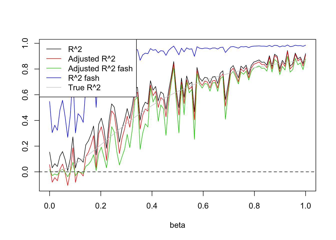
plot(trueR2,R2,type='l',ylim=range(c(R2,R2a,R2s,R2as,trueR2)))
lines(trueR2,R2a,col=2)
lines(trueR2,R2as,col=3)
lines(trueR2,R2s,col=4)
lines(trueR2,trueR2,col='grey80')
legend('topleft',c('R^2','Adjusted R^2','Adjusted R^2 fash','R^2 fash'),lty=c(1,1,1,1),col=c(1,2,3,4))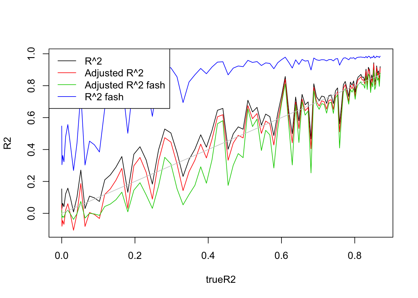
Compare fash and corshrink
1-d case
- \(n=100,p=1\)
Uniform(0,5):
library(CorShrink)
set.seed(1234)

n=100
p=1
R2=c()
R2a=c()
trueR2=c()

beta.list=seq(0,1,length.out = 100)
X=matrix(runif(n*(p),0,5),n,p)
for (i in 1:length(beta.list)) {
  beta=rep(beta.list[i],p)
  y=X*beta+rnorm(n)
  datax=data.frame(X=X,y=y)
  mod=lm(y~.,datax)
  mod.sy=summary(mod)
  R2[i]=mod.sy$r.squared
  R2a[i]=mod.sy$adj.r.squared
  trueR2[i]=1-(1)/(1+var(X%*%beta))
}
R2.fash=ash_r2(R2,n,p)
R2a.fash=ash_ar2(R2,n,p)
R2.cor=(CorShrinkVector(sqrt(R2),n))^2


plot(beta.list,R2,ylim=range(c(R2,R2a,R2s,R2as,trueR2)),main='',xlab='beta',ylab='',type='l')
lines(beta.list,R2a,col=2)
#lines(beta.list,R2a.fash,col=3)
lines(beta.list,R2.fash,col=3)
lines(beta.list,R2.cor,col=4)
lines(beta.list,trueR2,col='grey80')
abline(h=0,lty=2)
legend('topleft',c('R^2','Adjusted R^2','R^2 fash','R^2 CorShrink','True R^2'),lty=c(1,1,1,1,1),col=c(1,2,3,4,'grey80'))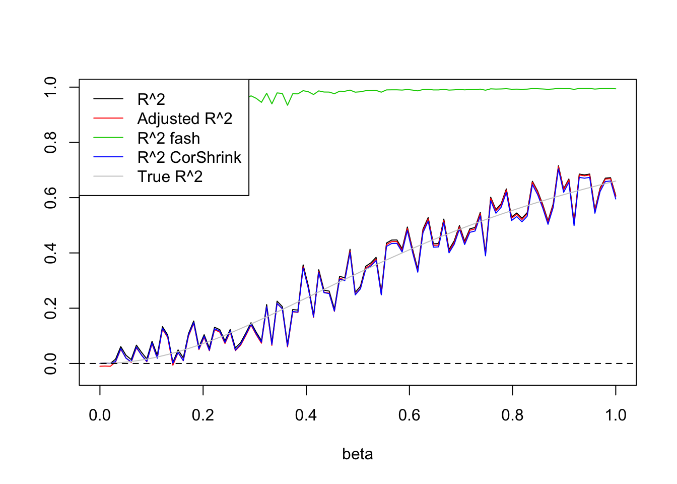
plot(trueR2,R2,type='l',ylim=range(c(R2,R2a,R2s,R2as,trueR2)))
lines(trueR2,R2a,col=2)
lines(trueR2,R2.fash,col=3)
lines(trueR2,R2.cor,col=4)
lines(trueR2,trueR2,col='grey80')
legend('topleft',c('R^2','Adjusted R^2','R^2 fash','R^2 CorShrink'),lty=c(1,1,1,1),col=c(1,2,3,4))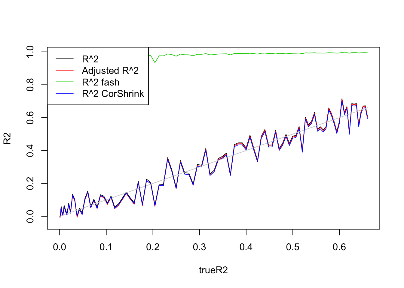
- \(n=30,p=1\)
Uniform(0,5):
set.seed(1234)

n=30
p=1
R2=c()
R2a=c()
trueR2=c()

beta.list=seq(0,1,length.out = 100)
X=matrix(runif(n*(p),0,5),n,p)
for (i in 1:length(beta.list)) {
  beta=rep(beta.list[i],p)
  y=X*beta+rnorm(n)
  datax=data.frame(X=X,y=y)
  mod=lm(y~.,datax)
  mod.sy=summary(mod)
  R2[i]=mod.sy$r.squared
  R2a[i]=mod.sy$adj.r.squared
  trueR2[i]=1-(1)/(1+var(X%*%beta))
}
R2.fash=ash_r2(R2,n,p)
R2a.fash=ash_ar2(R2,n,p)
R2.cor=(CorShrinkVector(sqrt(R2),n))^2


plot(beta.list,R2,ylim=range(c(R2,R2a,R2s,R2as,trueR2)),main='',xlab='beta',ylab='',type='l')
lines(beta.list,R2a,col=2)
#lines(beta.list,R2a.fash,col=3)
lines(beta.list,R2.fash,col=3)
lines(beta.list,R2.cor,col=4)
lines(beta.list,trueR2,col='grey80')
abline(h=0,lty=2)
legend('topleft',c('R^2','Adjusted R^2','R^2 fash','R^2 CorShrink','True R^2'),lty=c(1,1,1,1,1),col=c(1,2,3,4,'grey80'))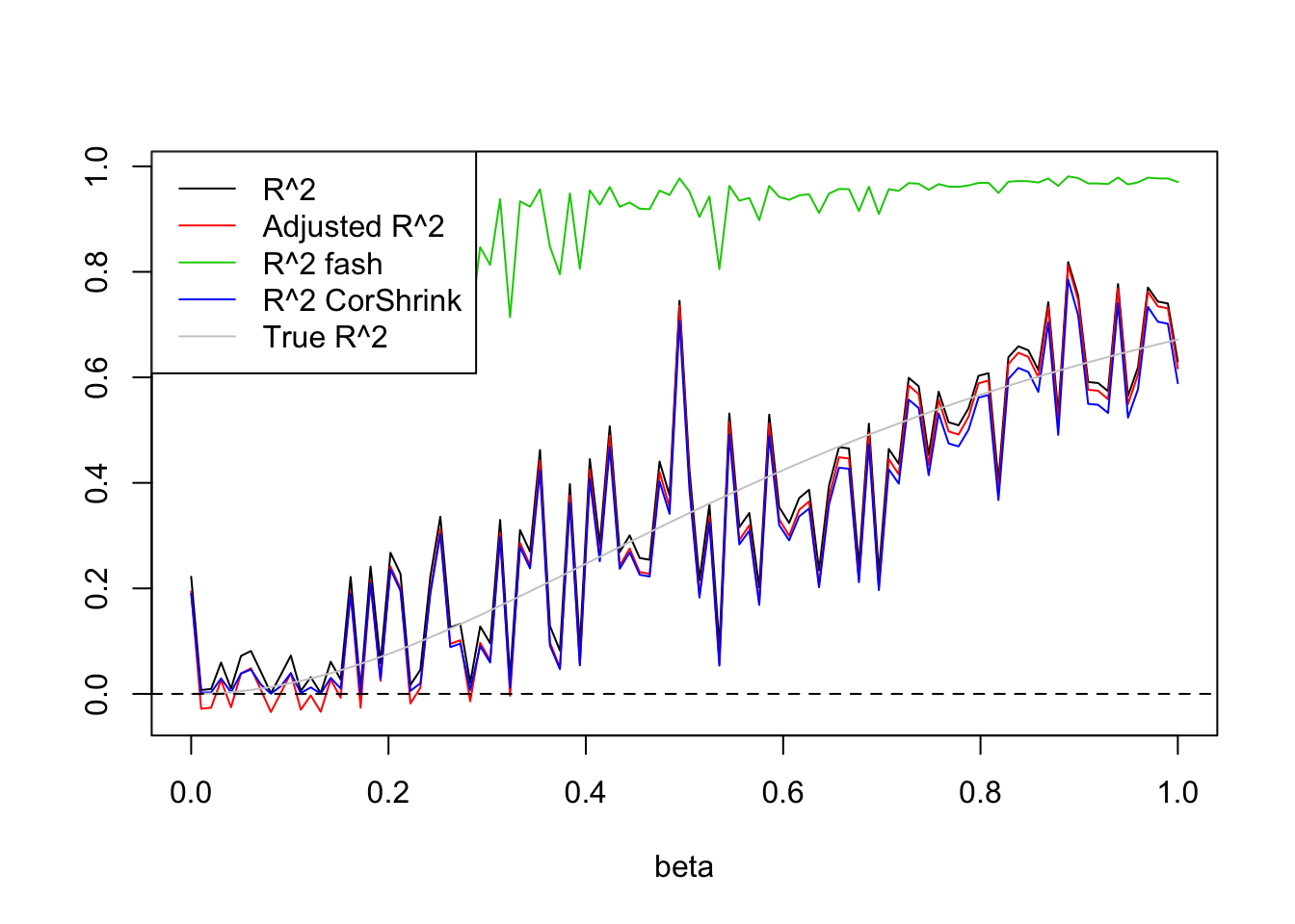
plot(trueR2,R2,type='l',ylim=range(c(R2,R2a,R2s,R2as,trueR2)))
lines(trueR2,R2a,col=2)
lines(trueR2,R2.fash,col=3)
lines(trueR2,R2.cor,col=4)
lines(trueR2,trueR2,col='grey80')
legend('topleft',c('R^2','Adjusted R^2','R^2 fash','R^2 CorShrink'),lty=c(1,1,1,1),col=c(1,2,3,4))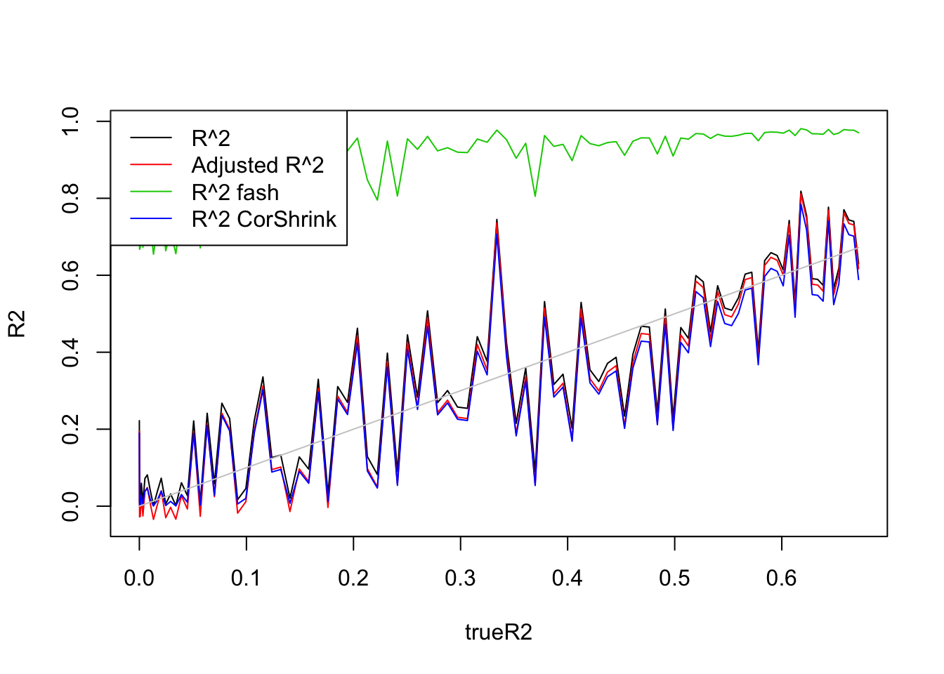
Multiple regression
- \(n=100, p=5\)
Uniform(0,2):
set.seed(1234)

n=100
p=5
R2=c()
R2a=c()
trueR2=c()

beta.list=seq(0,1,length.out = 100)
X=matrix(runif(n*(p),0,2),n,p)
for (i in 1:length(beta.list)) {
  beta=rep(beta.list[i],p)
  y=X%*%beta+rnorm(n)
  datax=data.frame(X=X,y=y)
  mod=lm(y~.,datax)
  mod.sy=summary(mod)
  R2[i]=mod.sy$r.squared
  R2a[i]=mod.sy$adj.r.squared
  trueR2[i]=1-(1)/(1+var(X%*%beta))
}
R2.fash=ash_r2(R2,n,p)
R2a.fash=ash_ar2(R2,n,p)
R2.cor=(CorShrinkVector(sqrt(R2),n))^2


plot(beta.list,R2,ylim=range(c(R2,R2a,R2s,R2as,trueR2)),main='',xlab='beta',ylab='',type='l')
lines(beta.list,R2a,col=2)
#lines(beta.list,R2a.fash,col=3)
lines(beta.list,R2.fash,col=3)
lines(beta.list,R2.cor,col=4)
lines(beta.list,trueR2,col='grey80')
abline(h=0,lty=2)
legend('topleft',c('R^2','Adjusted R^2','R^2 fash','R^2 CorShrink','True R^2'),lty=c(1,1,1,1,1),col=c(1,2,3,4,'grey80'))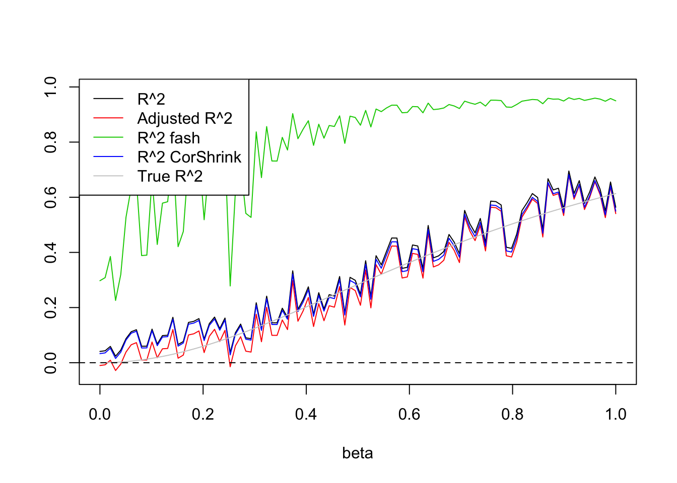
| Version | Author | Date |
|---|---|---|
| c6f9a91 | Dongyue Xie | 2019-02-10 |
plot(trueR2,R2,type='l',ylim=range(c(R2,R2a,R2s,R2as,trueR2)))
lines(trueR2,R2a,col=2)
lines(trueR2,R2.fash,col=3)
lines(trueR2,R2.cor,col=4)
lines(trueR2,trueR2,col='grey80')
legend('topleft',c('R^2','Adjusted R^2','R^2 fash','R^2 CorShrink'),lty=c(1,1,1,1),col=c(1,2,3,4))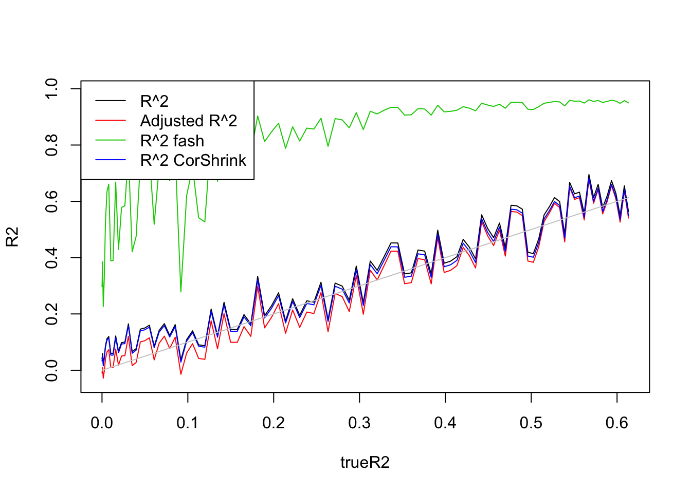
| Version | Author | Date |
|---|---|---|
| c6f9a91 | Dongyue Xie | 2019-02-10 |
- \(n=100,p=20\)
Uniform(0,1):
set.seed(1234)

n=100
p=20
R2=c()
R2a=c()
trueR2=c()

beta.list=seq(0,1,length.out = 100)
X=matrix(runif(n*(p),0,1),n,p)
for (i in 1:length(beta.list)) {
  beta=rep(beta.list[i],p)
  y=X%*%beta+rnorm(n)
  datax=data.frame(X=X,y=y)
  mod=lm(y~.,datax)
  mod.sy=summary(mod)
  R2[i]=mod.sy$r.squared
  R2a[i]=mod.sy$adj.r.squared
  trueR2[i]=1-(1)/(1+var(X%*%beta))
}
R2.fash=ash_r2(R2,n,p)
R2a.fash=ash_ar2(R2,n,p)
R2.cor=(CorShrinkVector(sqrt(R2),n))^2


plot(beta.list,R2,ylim=range(c(R2,R2a,R2s,R2as,trueR2)),main='',xlab='beta',ylab='',type='l')
lines(beta.list,R2a,col=2)
#lines(beta.list,R2a.fash,col=3)
lines(beta.list,R2.fash,col=3)
lines(beta.list,R2.cor,col=4)
lines(beta.list,trueR2,col='grey80')
abline(h=0,lty=2)
legend('topleft',c('R^2','Adjusted R^2','R^2 fash','R^2 CorShrink','True R^2'),lty=c(1,1,1,1,1),col=c(1,2,3,4,'grey80'))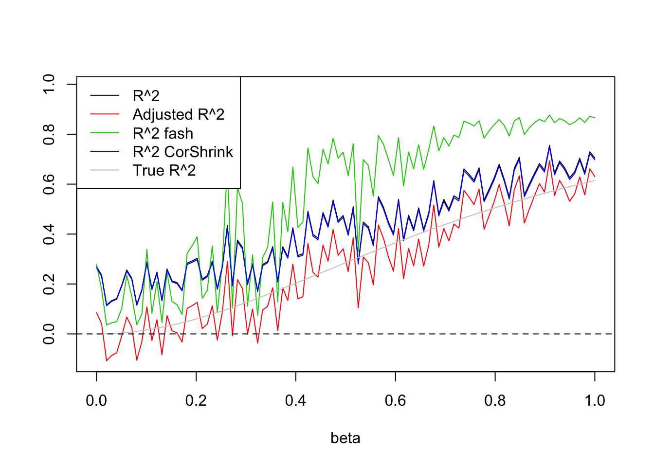
| Version | Author | Date |
|---|---|---|
| c6f9a91 | Dongyue Xie | 2019-02-10 |
plot(trueR2,R2,type='l',ylim=range(c(R2,R2a,R2s,R2as,trueR2)))
lines(trueR2,R2a,col=2)
lines(trueR2,R2.fash,col=3)
lines(trueR2,R2.cor,col=4)
lines(trueR2,trueR2,col='grey80')
legend('topleft',c('R^2','Adjusted R^2','R^2 fash','R^2 CorShrink'),lty=c(1,1,1,1),col=c(1,2,3,4))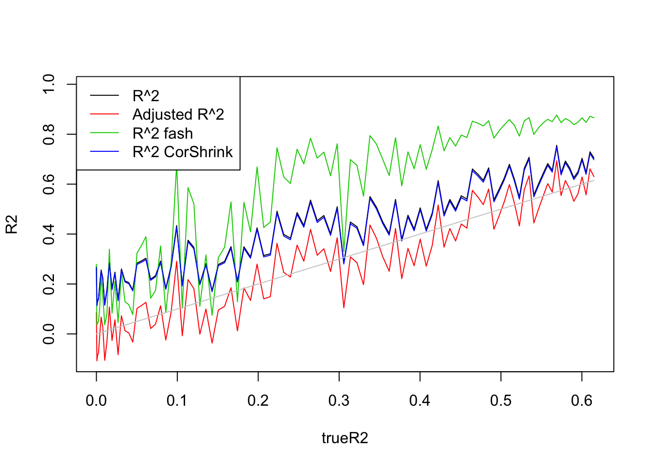
| Version | Author | Date |
|---|---|---|
| c6f9a91 | Dongyue Xie | 2019-02-10 |
\(n=100,p=50\)
Uniform(0,1):
set.seed(1234)

n=100
p=50
R2=c()
R2a=c()
trueR2=c()

beta.list=seq(0,1,length.out = 100)
X=matrix(runif(n*(p),0,1),n,p)
for (i in 1:length(beta.list)) {
  beta=rep(beta.list[i],p)
  y=X%*%beta+rnorm(n)
  datax=data.frame(X=X,y=y)
  mod=lm(y~.,datax)
  mod.sy=summary(mod)
  R2[i]=mod.sy$r.squared
  R2a[i]=mod.sy$adj.r.squared
  trueR2[i]=1-(1)/(1+var(X%*%beta))
}
R2.fash=ash_r2(R2,n,p)
R2a.fash=ash_ar2(R2,n,p)
R2.cor=(CorShrinkVector(sqrt(R2),n))^2


plot(beta.list,R2,ylim=range(c(R2,R2a,R2s,R2as,trueR2)),main='',xlab='beta',ylab='',type='l')
lines(beta.list,R2a,col=2)
#lines(beta.list,R2a.fash,col=3)
lines(beta.list,R2.fash,col=3)
lines(beta.list,R2.cor,col=4)
lines(beta.list,trueR2,col='grey80')
abline(h=0,lty=2)
legend('topleft',c('R^2','Adjusted R^2','R^2 fash','R^2 CorShrink','True R^2'),lty=c(1,1,1,1,1),col=c(1,2,3,4,'grey80'))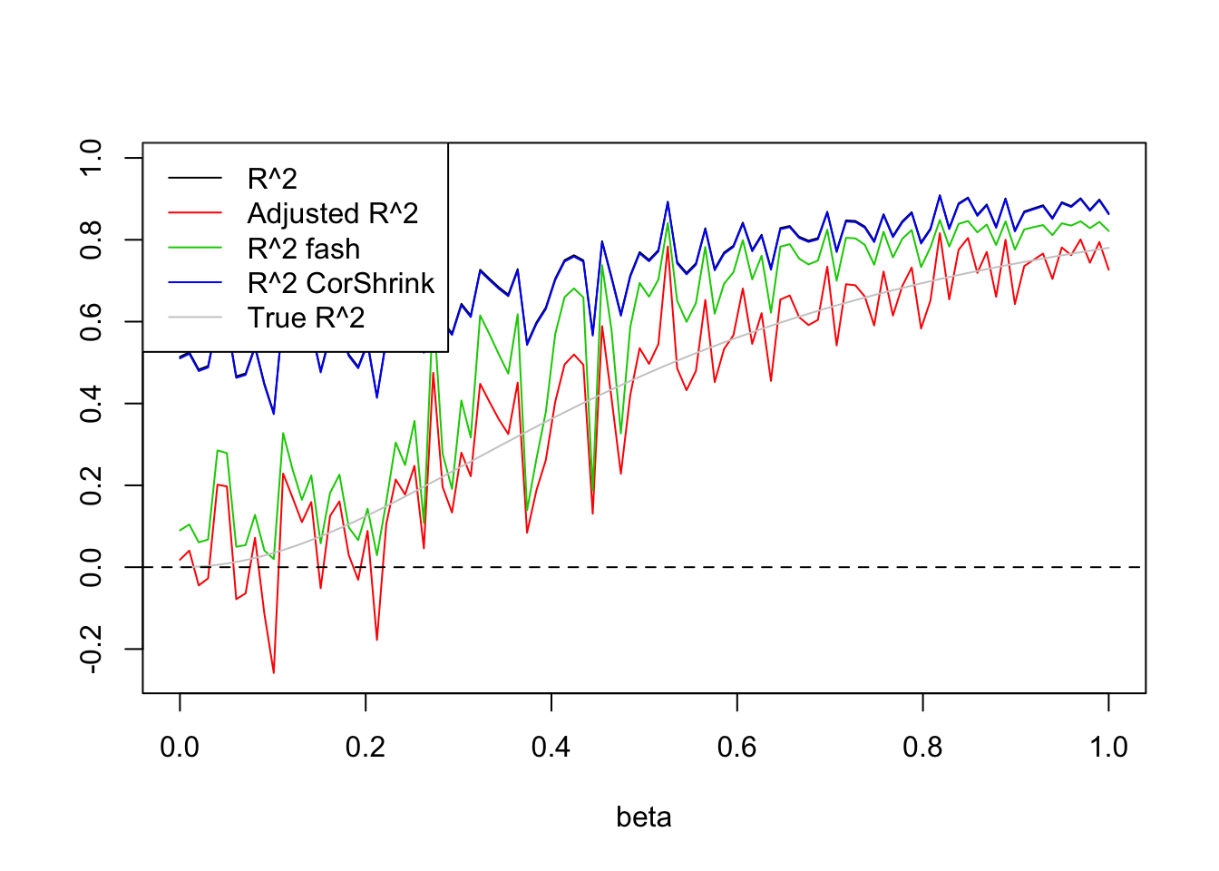
| Version | Author | Date |
|---|---|---|
| c6f9a91 | Dongyue Xie | 2019-02-10 |
plot(trueR2,R2,type='l',ylim=range(c(R2,R2a,R2s,R2as,trueR2)))
lines(trueR2,R2a,col=2)
lines(trueR2,R2.fash,col=3)
lines(trueR2,R2.cor,col=4)
lines(trueR2,trueR2,col='grey80')
legend('topleft',c('R^2','Adjusted R^2','R^2 fash','R^2 CorShrink'),lty=c(1,1,1,1),col=c(1,2,3,4))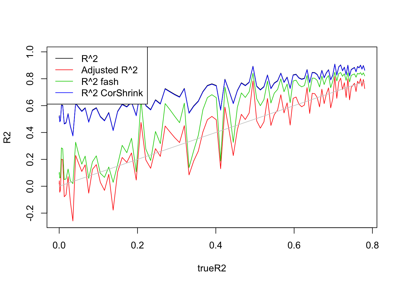
| Version | Author | Date |
|---|---|---|
| c6f9a91 | Dongyue Xie | 2019-02-10 |
- \(n=30, p=3\)
Uniform(0,5):
set.seed(1234)

n=30
p=3
R2=c()
R2a=c()
trueR2=c()

beta.list=seq(0,5,length.out = 100)
X=matrix(runif(n*(p),0,1),n,p)
for (i in 1:length(beta.list)) {
  beta=rep(beta.list[i],p)
  y=X%*%beta+rnorm(n)
  datax=data.frame(X=X,y=y)
  mod=lm(y~.,datax)
  mod.sy=summary(mod)
  R2[i]=mod.sy$r.squared
  R2a[i]=mod.sy$adj.r.squared
  trueR2[i]=1-(1)/(1+var(X%*%beta))
}
R2.fash=ash_r2(R2,n,p)
R2a.fash=ash_ar2(R2,n,p)
R2.cor=(CorShrinkVector(sqrt(R2),n))^2


plot(beta.list,R2,ylim=range(c(R2,R2a,R2s,R2as,trueR2)),main='',xlab='beta',ylab='',type='l')
lines(beta.list,R2a,col=2)
#lines(beta.list,R2a.fash,col=3)
lines(beta.list,R2.fash,col=3)
lines(beta.list,R2.cor,col=4)
lines(beta.list,trueR2,col='grey80')
abline(h=0,lty=2)
legend('topleft',c('R^2','Adjusted R^2','R^2 fash','R^2 CorShrink','True R^2'),lty=c(1,1,1,1,1),col=c(1,2,3,4,'grey80'))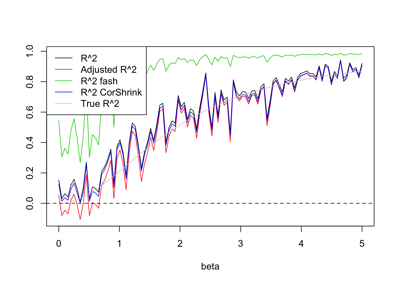
| Version | Author | Date |
|---|---|---|
| c6f9a91 | Dongyue Xie | 2019-02-10 |
plot(trueR2,R2,type='l',ylim=range(c(R2,R2a,R2s,R2as,trueR2)))
lines(trueR2,R2a,col=2)
lines(trueR2,R2.fash,col=3)
lines(trueR2,R2.cor,col=4)
lines(trueR2,trueR2,col='grey80')
legend('topleft',c('R^2','Adjusted R^2','R^2 fash','R^2 CorShrink'),lty=c(1,1,1,1),col=c(1,2,3,4))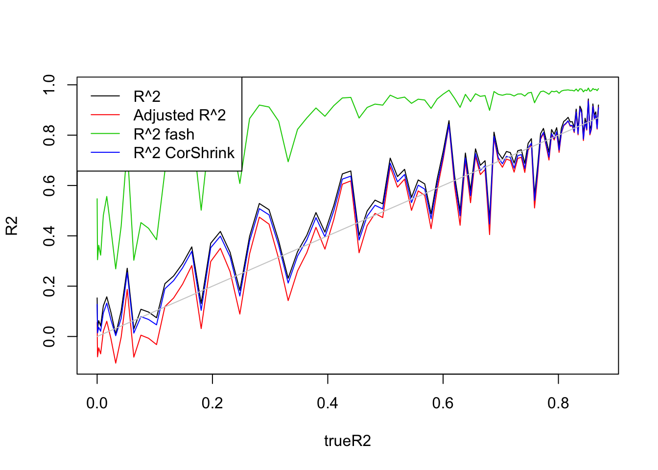
| Version | Author | Date |
|---|---|---|
| c6f9a91 | Dongyue Xie | 2019-02-10 |
Summary1
When generating X from Uniform(0,1), \(var(X\beta)\) is small and
fashcan shrink all \(R^2\) to 0. This happens when \(n,p\) are small. If \(p=20\), then this does not happen.CorShrink does not shrink \(R^2\). I can not really tell the difference from plots between Corshrink \(R^2\) and \(R&2\).
Adjusted \(R^2\) is a good shrinkage estimator of \(R^2\).
Sign of correlations
Randomize signs of \(R\) and see if corshrink gives the same results.
Random sample n/2 \(R^2\)s and set the sign of \(R\) to negative.
\(n=100,p=1\)
Uniform(0,1):
library(CorShrink)
set.seed(1234)

n=100
p=1
R2=c()
R2a=c()
trueR2=c()

beta.list=seq(0,1,length.out = 100)
X=matrix(runif(n*(p),0,5),n,p)
for (i in 1:length(beta.list)) {
  beta=rep(beta.list[i],p)
  y=X*beta+rnorm(n)
  datax=data.frame(X=X,y=y)
  mod=lm(y~.,datax)
  mod.sy=summary(mod)
  R2[i]=mod.sy$r.squared
  R2a[i]=mod.sy$adj.r.squared
  trueR2[i]=1-(1)/(1+var(X%*%beta))
}

R2.cor=(CorShrinkVector(sqrt(R2),n))^2
idx=sample(1:100,50)
R=sqrt(R2)
R[idx]=-R[idx]
R2.cor.sign=(CorShrinkVector(R,n))^2

plot(beta.list,R2,ylim=range(c(R2,R2.cor.sign,R2.cor,trueR2)),main='',xlab='beta',ylab='',type='l')
lines(beta.list,R2.cor,col=2)
lines(beta.list,R2.cor.sign,col=3)
lines(beta.list,trueR2,col='grey80')
abline(h=0,lty=2)
legend('topleft',c('R^2','R^2 CorShrink','R^2 CorShrink Random Sign','True R^2'),lty=c(1,1,1,1),col=c(1,2,3,'grey80'))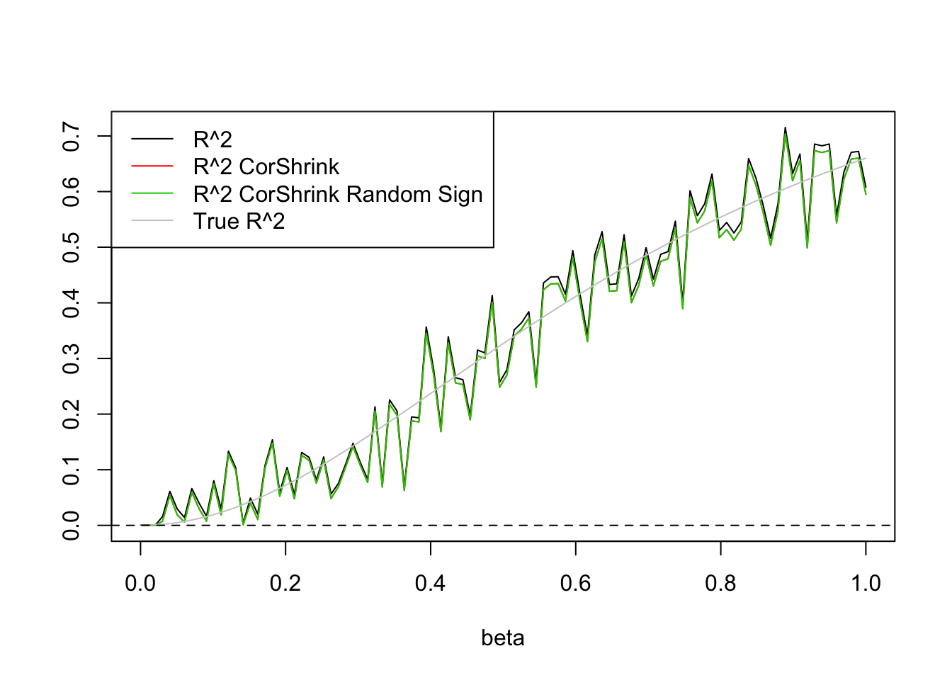
| Version | Author | Date |
|---|---|---|
| c6f9a91 | Dongyue Xie | 2019-02-10 |
plot(trueR2,R2,type='l',ylim=range(c(R2,R2.cor.sign,R2.cor,trueR2)))
lines(trueR2,R2.cor,col=2)
lines(trueR2,R2.cor.sign,col=3)
lines(trueR2,trueR2,col='grey80')
legend('topleft',c('R^2','R^2 CorShrink','R^2 CorShrink Random Sign'),lty=c(1,1,1),col=c(1,2,3))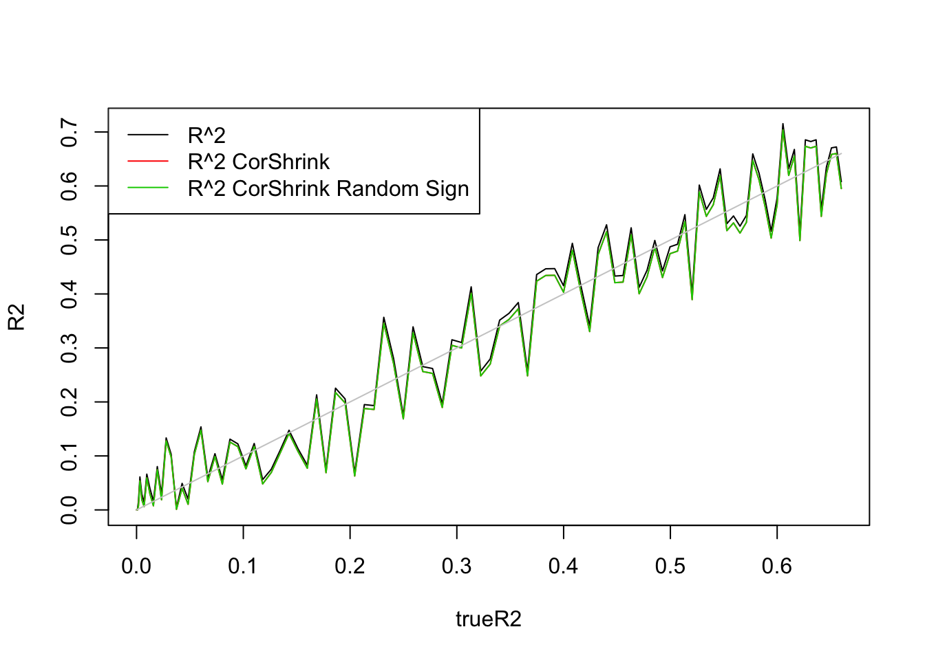
| Version | Author | Date |
|---|---|---|
| c6f9a91 | Dongyue Xie | 2019-02-10 |
So signs do not matter.
Estimates of g
Example 0
X from Uniform(0,5) and \(n=100,p=1\)
set.seed(1234)
n=100
p=1
R2=c()
R2a=c()
trueR2=c()
beta.list=seq(0,1,length.out = 100)
X=matrix(runif(n*(p),0,5),n,p)
for (i in 1:length(beta.list)) {
  beta=rep(beta.list[i],p)
  y=X%*%beta+rnorm(n)
  datax=data.frame(X=X,y=y)
  mod=lm(y~.,datax)
  mod.sy=summary(mod)
  R2[i]=mod.sy$r.squared
  R2a[i]=mod.sy$adj.r.squared
  trueR2[i]=1-(1)/(1+var(X%*%beta))
}

R2.fash=ash_r2(R2,n,p)
R2.cor=(CorShrinkVector(sqrt(R2),n))^2

plot(trueR2,R2.fash,type='l',ylim=range(c(R2.fash,R2.cor,trueR2)),ylab = '')
lines(trueR2,R2.cor,col=2)
lines(trueR2,trueR2,col='grey80')
legend('topleft',c('fash','Corshrink','True R2'),lty=c(1,1,1),col=c(1,2,'grey80'))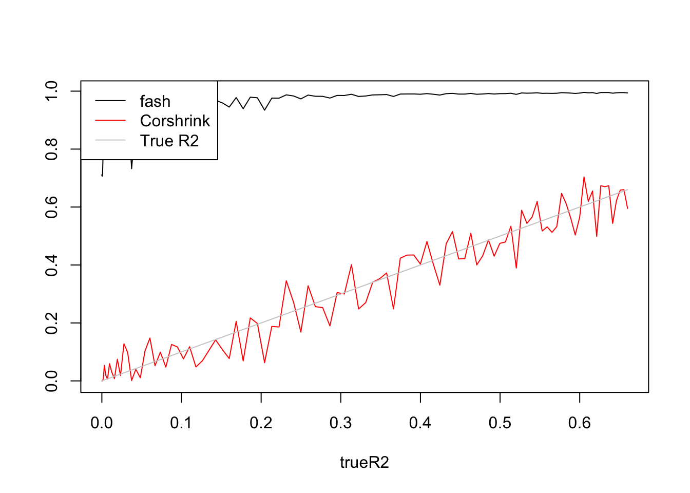
| Version | Author | Date |
|---|---|---|
| c6f9a91 | Dongyue Xie | 2019-02-10 |
fash:
log.ratio=log(1-R2)
ash.fit=ash(log.ratio,1,lik=lik_logF(df1=n-1,df2=n-1))
ash.fit$fitted_g
$pi
[1] 0.3941201 0.0000000 0.0000000 0.0000000 0.0000000 0.0000000 0.0000000
[8] 0.0000000 0.6058799 0.0000000
$a
[1] 0.00000000 -0.09507465 -0.13445586 -0.19014930 -0.26891172
[6] -0.38029861 -0.53782345 -0.76059722 -1.07564690 -1.52119443
$b
[1] 0.00000000 0.09507465 0.13445586 0.19014930 0.26891172 0.38029861
[7] 0.53782345 0.76059722 1.07564690 1.52119443
attr(,"class")
[1] "unimix"
attr(,"row.names")
[1] 1 2 3 4 5 6 7 8 9 10Fitted g concentrates at \(0.4*\delta_0+0.6*Uniform(-1.07,1.07)\)
Corshrink:
R=sqrt(R2)
corvec=R
corvec_trans = 0.5 * log((1 + corvec)/(1 - corvec))
corvec_trans_sd = rep(sqrt(1/(n - 1) + 2/(n -
            1)^2), length(corvec_trans))

ash.control=list()
ash.control.default = list(pointmass = TRUE, mixcompdist = "normal",
        nullweight = 10, fixg = FALSE, mode = 0, optmethod = "mixEM",
        prior = "nullbiased", gridmult = sqrt(2), outputlevel = 2,
        alpha = 0, df = NULL, control = list(K = 1, method = 3,
            square = TRUE, step.min0 = 1, step.max0 = 1, mstep = 4,
            kr = 1, objfn.inc = 1, tol = 1e-05,
            trace = FALSE))
ash.control <- utils::modifyList(ash.control.default, ash.control)


fit = do.call(ashr::ash, append(list(betahat = corvec_trans,
        sebetahat = corvec_trans_sd), ash.control))
fit$fitted_g
$pi
[1] 1.198336e-01 3.102514e-09 3.098655e-09 3.055578e-09 2.825173e-09
[6] 1.905128e-09 2.187591e-09 7.621847e-08 3.302451e-07 3.196176e-09
[11] 0.000000e+00 0.000000e+00 9.715355e-07 5.124079e-01 3.677565e-01
[16] 5.913347e-07 0.000000e+00 0.000000e+00
$mean
[1] 0 0 0 0 0 0 0 0 0 0 0 0 0 0 0 0 0 0
$sd
[1] 0.000000000 0.009663507 0.013666263 0.019327015 0.027332527
[6] 0.038654030 0.054665053 0.077308060 0.109330107 0.154616120
[11] 0.218660214 0.309232240 0.437320427 0.618464480 0.874640855
[16] 1.236928959 1.749281710 2.473857919
attr(,"class")
[1] "normalmix"
attr(,"row.names")
[1] 1 2 3 4 5 6 7 8 9 10 11 12 13 14 15 16 17 18Fitted g concentrates at \(0.12*\delta_0+0.5*N(0,0.62^2)+0.37*N(0,0.87^2)\)
Example 1
X from Uniform(0,1) and \(n=100,p=5\)
set.seed(1234)
n=100
p=5
R2=c()
R2a=c()
trueR2=c()
beta.list=seq(0,1,length.out = 100)
X=matrix(runif(n*(p),0,1),n,p)
for (i in 1:length(beta.list)) {
  beta=rep(beta.list[i],p)
  y=X%*%beta+rnorm(n)
  datax=data.frame(X=X,y=y)
  mod=lm(y~.,datax)
  mod.sy=summary(mod)
  R2[i]=mod.sy$r.squared
  R2a[i]=mod.sy$adj.r.squared
  trueR2[i]=1-(1)/(1+var(X%*%beta))
}

R2.fash=ash_r2(R2,n,p)
R2.cor=(CorShrinkVector(sqrt(R2),n))^2

plot(trueR2,R2.fash,type='l',ylim=range(c(R2.fash,R2.cor,trueR2)),ylab = '')
lines(trueR2,R2.cor,col=2)
lines(trueR2,trueR2,col='grey80')
legend('topleft',c('fash','Corshrink','True R2'),lty=c(1,1,1),col=c(1,2,'grey80'))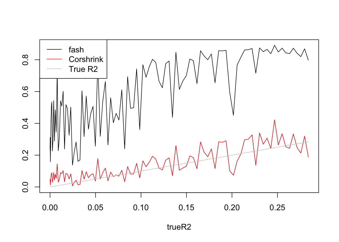
| Version | Author | Date |
|---|---|---|
| c6f9a91 | Dongyue Xie | 2019-02-10 |
fash:
log.ratio=log(1-R2)
ash.fit=ash(log.ratio,1,lik=lik_logF(df1=n-1,df2=n-1))
ash.fit$fitted_g
$pi
[1] 1 0 0 0 0 0 0 0
$a
[1] 0.0000000 -0.1000000 -0.1414214 -0.2000000 -0.2828427 -0.4000000
[7] -0.5656854 -0.8000000
$b
[1] 0.0000000 0.1000000 0.1414214 0.2000000 0.2828427 0.4000000 0.5656854
[8] 0.8000000
attr(,"class")
[1] "unimix"
attr(,"row.names")
[1] 1 2 3 4 5 6 7 8Fitted g is at point mass at 0.
Corshrink:
R=sqrt(R2)
corvec=R
corvec_trans = 0.5 * log((1 + corvec)/(1 - corvec))
corvec_trans_sd = rep(sqrt(1/(n - 1) + 2/(n -
            1)^2), length(corvec_trans))

ash.control=list()
ash.control.default = list(pointmass = TRUE, mixcompdist = "normal",
        nullweight = 10, fixg = FALSE, mode = 0, optmethod = "mixEM",
        prior = "nullbiased", gridmult = sqrt(2), outputlevel = 2,
        alpha = 0, df = NULL, control = list(K = 1, method = 3,
            square = TRUE, step.min0 = 1, step.max0 = 1, mstep = 4,
            kr = 1, objfn.inc = 1, tol = 1e-05,
            trace = FALSE))
ash.control <- utils::modifyList(ash.control.default, ash.control)


fit = do.call(ashr::ash, append(list(betahat = corvec_trans,
        sebetahat = corvec_trans_sd), ash.control))
fit$fitted_g
$pi
[1] 9.802685e-02 3.574714e-08 3.546272e-08 3.428903e-08 2.954403e-08
[6] 1.308498e-08 5.872701e-09 2.297127e-07 0.000000e+00 0.000000e+00
[11] 0.000000e+00 0.000000e+00 9.018827e-01 8.912271e-05 1.659427e-14
[16] 9.609965e-07 0.000000e+00
$mean
[1] 0 0 0 0 0 0 0 0 0 0 0 0 0 0 0 0 0
$sd
[1] 0.000000000 0.009016022 0.012750581 0.018032044 0.025501162
[6] 0.036064089 0.051002323 0.072128177 0.102004647 0.144256355
[11] 0.204009293 0.288512709 0.408018586 0.577025418 0.816037173
[16] 1.154050837 1.632074345
attr(,"class")
[1] "normalmix"
attr(,"row.names")
[1] 1 2 3 4 5 6 7 8 9 10 11 12 13 14 15 16 17Fitted g concentrates at \(0.9*N(0,0.41^2)\)
Example 2
X from Uniform(0,5) and \(n=100,p=5\)
set.seed(1234)
n=100
p=5
R2=c()
R2a=c()
trueR2=c()

beta.list=seq(0,1,length.out = 100)
X=matrix(runif(n*(p),0,5),n,p)
for (i in 1:length(beta.list)) {
  beta=rep(beta.list[i],p)
  y=X%*%beta+rnorm(n)
  datax=data.frame(X=X,y=y)
  mod=lm(y~.,datax)
  mod.sy=summary(mod)
  R2[i]=mod.sy$r.squared
  R2a[i]=mod.sy$adj.r.squared
  trueR2[i]=1-(1)/(1+var(X%*%beta))
}

R2.fash=ash_r2(R2,n,p)
R2.cor=(CorShrinkVector(sqrt(R2),n))^2

plot(trueR2,R2.fash,type='l',ylim=range(c(R2.fash,R2.cor,trueR2)),ylab='')
lines(trueR2,R2.cor,col=2)
lines(trueR2,trueR2,col='grey80')
legend('topleft',c('fash','Corshrink','True R2'),lty=c(1,1,1),col=c(1,2,'grey80'))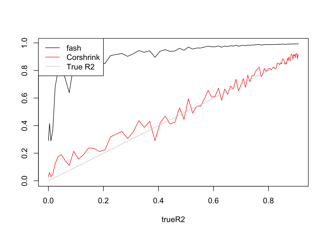
| Version | Author | Date |
|---|---|---|
| c6f9a91 | Dongyue Xie | 2019-02-10 |
fash:
log.ratio=log(1-R2)
ash.fit=ash(log.ratio,1,lik=lik_logF(df1=n-1,df2=n-1))
ash.fit$fitted_g
$pi
[1] 0.192508 0.000000 0.000000 0.000000 0.000000 0.000000 0.000000
[8] 0.000000 0.000000 0.000000 0.000000 0.807492 0.000000 0.000000
$a
[1] 0.00000000 -0.07447264 -0.10532021 -0.14894527 -0.21064043
[6] -0.29789055 -0.42128085 -0.59578110 -0.84256171 -1.19156219
[11] -1.68512342 -2.38312439 -3.37024683 -4.76624878
$b
[1] 0.00000000 0.07447264 0.10532021 0.14894527 0.21064043 0.29789055
[7] 0.42128085 0.59578110 0.84256171 1.19156219 1.68512342 2.38312439
[13] 3.37024683 4.76624878
attr(,"class")
[1] "unimix"
attr(,"row.names")
[1] 1 2 3 4 5 6 7 8 9 10 11 12 13 14Fitted g concentrates at \(0.19*\delta_0+0.81*Uniform(-2.38,2.38)\).
Corshrink:
R=sqrt(R2)
corvec=R
corvec_trans = 0.5 * log((1 + corvec)/(1 - corvec))
corvec_trans_sd = rep(sqrt(1/(n - 1) + 2/(n -
            1)^2), length(corvec_trans))

ash.control=list()
ash.control.default = list(pointmass = TRUE, mixcompdist = "normal",
        nullweight = 10, fixg = FALSE, mode = 0, optmethod = "mixEM",
        prior = "nullbiased", gridmult = sqrt(2), outputlevel = 2,
        alpha = 0, df = NULL, control = list(K = 1, method = 3,
            square = TRUE, step.min0 = 1, step.max0 = 1, mstep = 4,
            kr = 1, objfn.inc = 1, tol = 1e-05,
            trace = FALSE))
ash.control <- utils::modifyList(ash.control.default, ash.control)


fit = do.call(ashr::ash, append(list(betahat = corvec_trans,
        sebetahat = corvec_trans_sd), ash.control))
fit$fitted_g
$pi
[1] 8.739018e-02 1.585320e-10 1.795248e-10 2.290505e-10 3.656616e-10
[6] 8.673704e-10 3.820458e-09 3.574858e-08 5.461574e-07 5.361614e-06
[11] 2.307459e-06 8.830531e-07 2.605247e-06 4.894297e-07 0.000000e+00
[16] 5.058173e-06 9.125923e-01 2.335972e-07 0.000000e+00 0.000000e+00
$mean
[1] 0 0 0 0 0 0 0 0 0 0 0 0 0 0 0 0 0 0 0 0
$sd
[1] 0.000000000 0.007669231 0.010845930 0.015338461 0.021691860
[6] 0.030676923 0.043383720 0.061353845 0.086767440 0.122707690
[11] 0.173534880 0.245415381 0.347069760 0.490830762 0.694139520
[16] 0.981661524 1.388279041 1.963323048 2.776558081 3.926646095
attr(,"class")
[1] "normalmix"
attr(,"row.names")
[1] 1 2 3 4 5 6 7 8 9 10 11 12 13 14 15 16 17 18 19 20Fitted g concentrates at \(0.91*N(0,1.39^2)\)
Summary2
Fash uses a mixture of point mass and uniform distributions as prior while CorShrink uses a mixture of point mass and normal distirbutions. Fash in these examples put more weights on point mass in fitted g than CorShrink.
Thoughts
Applying
fashto shrink \(R^2\) replies on F distribution, which is from the ratio of two variances. F distribution replies on normal assumption and independence of two normal populations. However, \(var(\sigma^2)\) and \(var(y)=var(X\beta)+var(\sigma^2)\) are not independent. So rigourously speaking, usingfashis not appropriate here.Corshirnkdepends on Fisher transformation which has bivariate normal assumption. Since \(R^2=r^2_{y,\hat y}\), we can applyCorshirnkif \(y,\hat y\) is bivariate normal distributed. By saying \(y,\hat y\) is bivariate normal distributed, I mean \(y,\hat y\) are \(n\) i.i.d samples from a bivariate normal distribution. However, this can hardly be true because \(\hat y=Hy\) where \(H=X(X^TX)^{-1}X^T\), so the \(n\) samples \(y,\hat y\) are not independently generated.From the examples above, adjusted \(R^2\) is a good estimate of true \(R^2\). It gives estimate close to ture \(R^2\) which can be seen from the True \(R^2\) - estimated \(R^2\) plot. It’s pitfall it that it’s no longer necessatily positive - it can be negative.
sessionInfo()R version 3.6.1 (2019-07-05)
Platform: x86_64-apple-darwin15.6.0 (64-bit)
Running under: macOS High Sierra 10.13.6
Matrix products: default
BLAS: /Library/Frameworks/R.framework/Versions/3.6/Resources/lib/libRblas.0.dylib
LAPACK: /Library/Frameworks/R.framework/Versions/3.6/Resources/lib/libRlapack.dylib
locale:
[1] en_US.UTF-8/en_US.UTF-8/en_US.UTF-8/C/en_US.UTF-8/en_US.UTF-8
attached base packages:
[1] stats graphics grDevices utils datasets methods base
other attached packages:
[1] CorShrink_0.1-6 ashr_2.2-38
loaded via a namespace (and not attached):
[1] gmp_0.6-0 Rcpp_1.0.2 plyr_1.8.4
[4] compiler_3.6.1 later_1.0.0 git2r_0.26.1
[7] CVXR_1.0-1 workflowr_1.5.0 iterators_1.0.12
[10] tools_3.6.1 corrplot_0.84 bit_1.1-14
[13] digest_0.6.21 gtable_0.3.0 evaluate_0.14
[16] lattice_0.20-38 rlang_0.4.5 Matrix_1.2-17
[19] foreach_1.4.7 yaml_2.2.0 parallel_3.6.1
[22] xfun_0.10 gridExtra_2.3 Rmpfr_0.8-1
[25] stringr_1.4.0 knitr_1.25 fs_1.3.1
[28] glmnet_2.0-18 bit64_0.9-7 rprojroot_1.3-2
[31] grid_3.6.1 glue_1.3.1 R6_2.4.0
[34] rmarkdown_1.16 mixsqp_0.1-97 reshape2_1.4.3
[37] corpcor_1.6.9 magrittr_1.5 whisker_0.4
[40] backports_1.1.5 promises_1.1.0 codetools_0.2-16
[43] htmltools_0.4.0 MASS_7.3-51.4 httpuv_1.5.2
[46] stringi_1.4.3 doParallel_1.0.15 pscl_1.5.2
[49] truncnorm_1.0-8 SQUAREM_2017.10-1