Variance stablizing transformation

workflowr

• Summary
• Checks
• Past versions

Last updated: 2020-09-07

Checks: 7 0

Knit directory: smash-gen/

This reproducible R Markdown analysis was created with workflowr (version 1.5.0). The Checks tab describes the reproducibility checks that were applied when the results were created. The Past versions tab lists the development history.

---

R Markdown file: up-to-date

Great! Since the R Markdown file has been committed to the Git repository, you know the exact version of the code that produced these results.

Environment: empty

Great job! The global environment was empty. Objects defined in the global environment can affect the analysis in your R Markdown file in unknown ways. For reproduciblity it’s best to always run the code in an empty environment.

Seed: set.seed(20180501)

The command set.seed(20180501) was run prior to running the code in the R Markdown file. Setting a seed ensures that any results that rely on randomness, e.g. subsampling or permutations, are reproducible.

Session information: recorded

Great job! Recording the operating system, R version, and package versions is critical for reproducibility.

Cache: none

Nice! There were no cached chunks for this analysis, so you can be confident that you successfully produced the results during this run.

File paths: relative

Great job! Using relative paths to the files within your workflowr project makes it easier to run your code on other machines.

Repository version: 0f60dad

Great! You are using Git for version control. Tracking code development and connecting the code version to the results is critical for reproducibility. The version displayed above was the version of the Git repository at the time these results were generated.

Note that you need to be careful to ensure that all relevant files for the analysis have been committed to Git prior to generating the results (you can use wflow_publish or wflow_git_commit). workflowr only checks the R Markdown file, but you know if there are other scripts or data files that it depends on. Below is the status of the Git repository when the results were generated:

Ignored files:
    Ignored:    .DS_Store
    Ignored:    .Rhistory
    Ignored:    .Rproj.user/
    Ignored:    data/.DS_Store

Untracked files:
    Untracked:  analysis/pln_smooth.Rmd
    Untracked:  analysis/smashadditive.Rmd
    Untracked:  analysis/talk1011.Rmd
    Untracked:  talk.Rmd
    Untracked:  talk.html
    Untracked:  talk.pdf

Unstaged changes:
    Modified:   analysis/binomial.Rmd
    Modified:   analysis/chipexo.Rmd
    Modified:   analysis/fda.Rmd
    Modified:   analysis/index.Rmd
    Modified:   analysis/protein.Rmd
    Modified:   analysis/r2.Rmd
    Modified:   analysis/sigma.Rmd

Note that any generated files, e.g. HTML, png, CSS, etc., are not included in this status report because it is ok for generated content to have uncommitted changes.

---

These are the previous versions of the R Markdown and HTML files. If you’ve configured a remote Git repository (see ?wflow_git_remote), click on the hyperlinks in the table below to view them.

File	Version	Author	Date	Message
Rmd	0f60dad	Dongyue Xie	2020-09-08	wflow_publish(“analysis/vst.Rmd”)
html	7386626	Dongyue Xie	2018-10-23	Build site.
Rmd	4ae0ded	Dongyue Xie	2018-10-23	wflow_publish(“analysis/vst.Rmd”)
html	a9755fb	Dongyue Xie	2018-10-18	Build site.
Rmd	adaace5	Dongyue Xie	2018-10-18	wflow_publish(“analysis/vst.Rmd”)
html	d45f4a0	Dongyue Xie	2018-10-16	Build site.
Rmd	4c8fd13	Dongyue Xie	2018-10-16	vst analysis
html	50eeda4	Dongyue Xie	2018-10-16	Build site.
Rmd	ce75cae	Dongyue Xie	2018-10-16	vst analysis
html	e24d0a7	Dongyue Xie	2018-10-16	Build site.
Rmd	0d956ea	Dongyue Xie	2018-10-16	vst analysis

---

Introduction

Variance stablizing transformation.

\(E(X)=\mu\) and \(Var(X)=g(\mu)\), want to find \(f(\cdot)\) s.t \(Var(f(X))\) has constant variance. Consider the Taylor series expansion of \(f(X)\) around \(\mu\): \(f(X)\approx f(\mu)+(Y-\mu)f'(\mu)\) so we have \([f(X)-f(\mu)]^2\approx (X-\mu)^2(f'(\mu))^2 \Rightarrow Var(f(X))\approx Var(X)(f'(\mu))^2\).

For poisson distribution, \((f'(\mu))^2\propto \mu^{-1}\) so if we take \(Y=\sqrt{X}\) then \(Var(Y)\approx \frac{1}{4}\). This was original proposed by Bartlett in 1936.

For Binomial data, \((f'(\mu))^2\propto 1/(np(1-p))\) so if we take \(Y=sin^{-1}(\sqrt{X/n})\) then \(Var(Y)\approx \frac{1}{2}\).

Anscombe(1948) shows that for \(Y=\sqrt{X+c}\), \(Var(Y)\approx \frac{1}{4}[1+\frac{3-8c}{8\mu}+\frac{32c^2-52c+17}{2\mu^2}]]\). If take \(c=3/8\) and for large \(\mu\), \(Var(Y)\approx 1/4\). Also clearly, \(\lim_{\mu\to 0}Var(\sqrt{X+c})=0\).

mu=seq(0,10,length.out = 500)
ans=c()
sr=c()
set.seed(12345)
for (i  in 1:500) {
  x=rpois(1e6,mu[i])
  ans[i]=var(sqrt(x+3/8))
  sr[i]=var(sqrt(x))
}
plot(mu,ans,type='l',ylim=c(0,0.5),ylab='')
lines(mu,sr,col=4)
abline(a=0.25,b=0,lty=2)
legend('bottomright',c('anscombe','square root'),lty=c(1,1),col=c(1,4))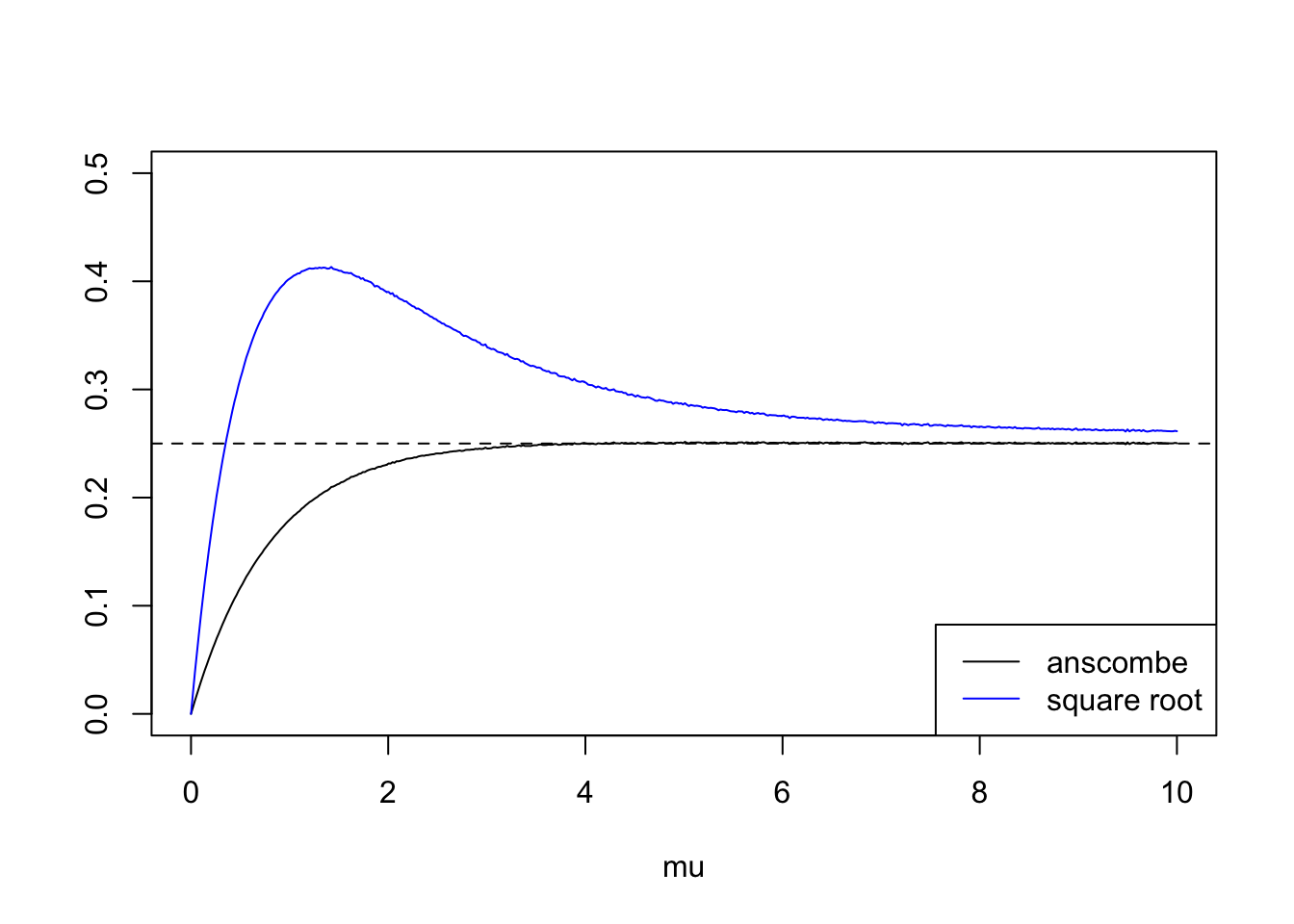

Past versions of unnamed-chunk-1-1.png

Version	Author	Date
e24d0a7	Dongyue Xie	2018-10-16

Apprently, if the mean is small say 1 or 2 then the transformed variable has variance smaller than 0.25. One way to adjust for small counts is to take all possibilities into account. For example, if we observe x=0, then we can assign the following variance to its transformation, let \(y\sim Poisson(\lambda)\): \(\frac{\int p(x=0;\lambda)var(\sqrt{y+c};\lambda)d\lambda}{\int p(x=0;\lambda)d\lambda}\). In practice we can generate a grid of discrete values and evaluate the above quantity.

for(i in c(0,1,2)){
 p0 = dpois(i,mu)
 p0 = p0/sum(p0)
 p0 = sum(p0*ans)
 print(p0)
}

[1] 0.1382905
[1] 0.2018222
[1] 0.2293388

Compare log and anscombe transformation

Poisson variance stablizing trasformations: square root and Anscombe transformation.

For vst, if we observe \(x=0\), then I use \(var(\sqrt{X+3/8})=0\) instead of \(1/4\).

vst_smooth=function(x,method,ep=1e-5){
  n=length(x)
  if(method=='sr'){
    x.t=sqrt(x)
    x.var=rep(1/4,n)
    x.var[x==0]=0
    mu.hat=(smashr::smash.gaus(x.t,sigma=sqrt(x.var)))^2
    
  }
  if(method=='anscombe'){
    x.t=sqrt(x+3/8)
    x.var=rep(1/4,n)
    x.var[x==0]=0
    mu.hat=(smashr::smash.gaus(x.t,sigma=sqrt(x.var)))^2-3/8
  }
  if(method=='log'){
    x.t=x
    x.t[x==0]=ep
    x.var=1/x.t
    x.t=log(x.t)
    mu.hat=exp(smashr::smash.gaus(x.t,sigma=sqrt(x.var)))
  }
  return(mu.hat)
}

simu_study=function(m,sig=0,nsimu=30,seed=12345){
  set.seed(seed)
  sr=c()
  an=c()
  ashp=c()
  for (i in 1:nsimu) {
    lambda=exp(log(m)+rnorm(n,0,sig))
    x=rpois(n,lambda)
    mu.sr=vst_smooth(x,'sr')
    mu.an=vst_smooth(x,'anscombe')
    mu.ash=smash_gen_lite(x,sigma = sig)
    sr=rbind(sr,mu.sr)
    an=rbind(an,mu.an)
    ashp=rbind(ashp,mu.ash)
  }
  return(list(sr=sr,an=an,ashp=ashp))
}

When there are a number of \(0s\) in the observation: (mean function (0.1,6))

library(ashr)
library(smashrgen)
spike.f = function(x) (0.75 * exp(-500 * (x - 0.23)^2) + 1.5 * exp(-2000 * (x - 0.33)^2) + 3 * exp(-8000 * (x - 0.47)^2) + 2.25 * exp(-16000 * 
    (x - 0.69)^2) + 0.5 * exp(-32000 * (x - 0.83)^2))
n = 512
t = 1:n/n
m = spike.f(t)

m=m*2+0.1
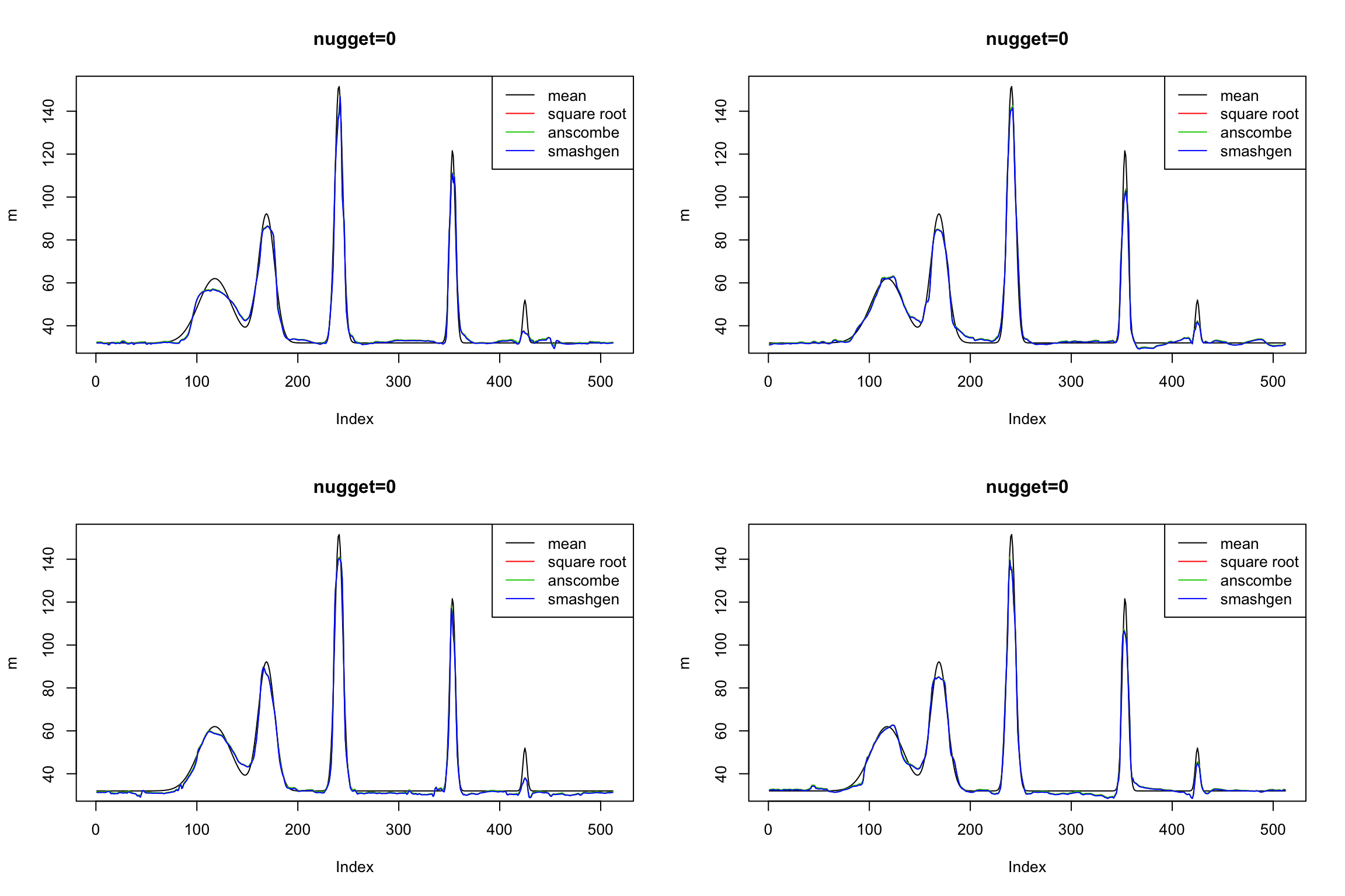
range(m)

[1] 0.100000 6.076316

result=simu_study(m)


mses=lapply(result, function(x){apply(x, 1, function(y){mean((y-m)^2)})})

par(mfrow=c(2,2))

for (j in 1:4) {
  plot(m,type='l',main='nugget=0')
lines(result$sr[j,],col=2)
lines(result$an[j,],col=3)
lines(result$ashp[j,],col=4)
legend('topright',c('mean','square root','anscombe','smashgen'),lty=c(1,1,1,1),col=c(1,2,3,4))

}

Past versions of unnamed-chunk-5-1.png

Version	Author	Date
7386626	Dongyue Xie	2018-10-23
d45f4a0	Dongyue Xie	2018-10-16
e24d0a7	Dongyue Xie	2018-10-16

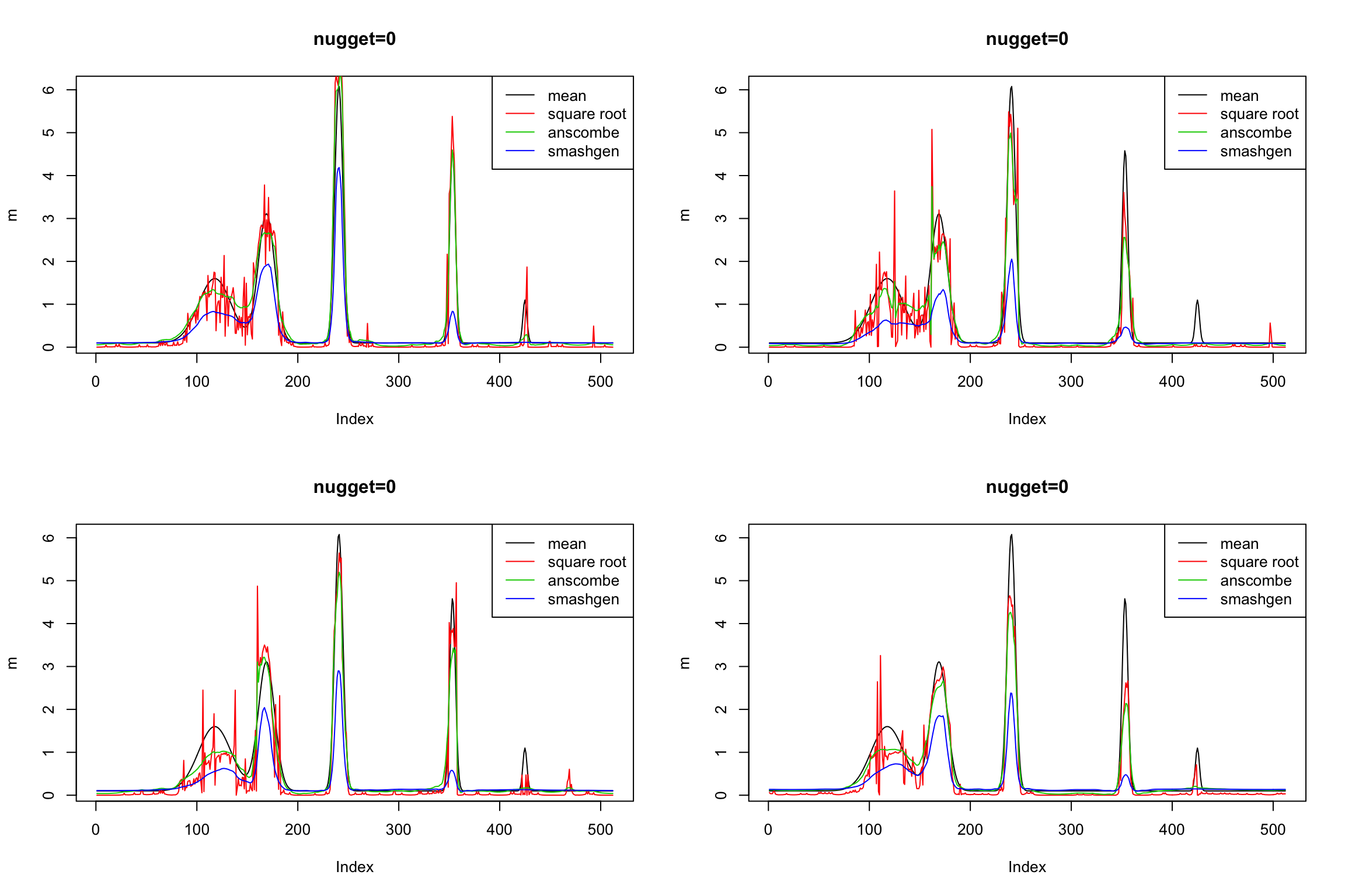
boxplot(mses,names = c('square root','anscombe','smashgen'),main='nugget=0',ylab='MSE')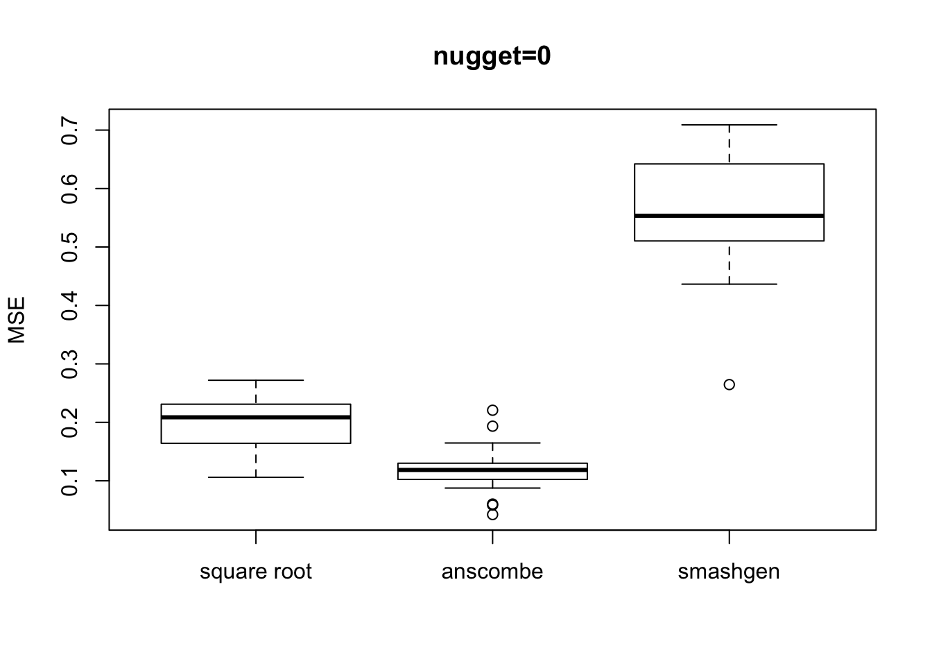

Past versions of unnamed-chunk-6-1.png

Version	Author	Date
7386626	Dongyue Xie	2018-10-23

########
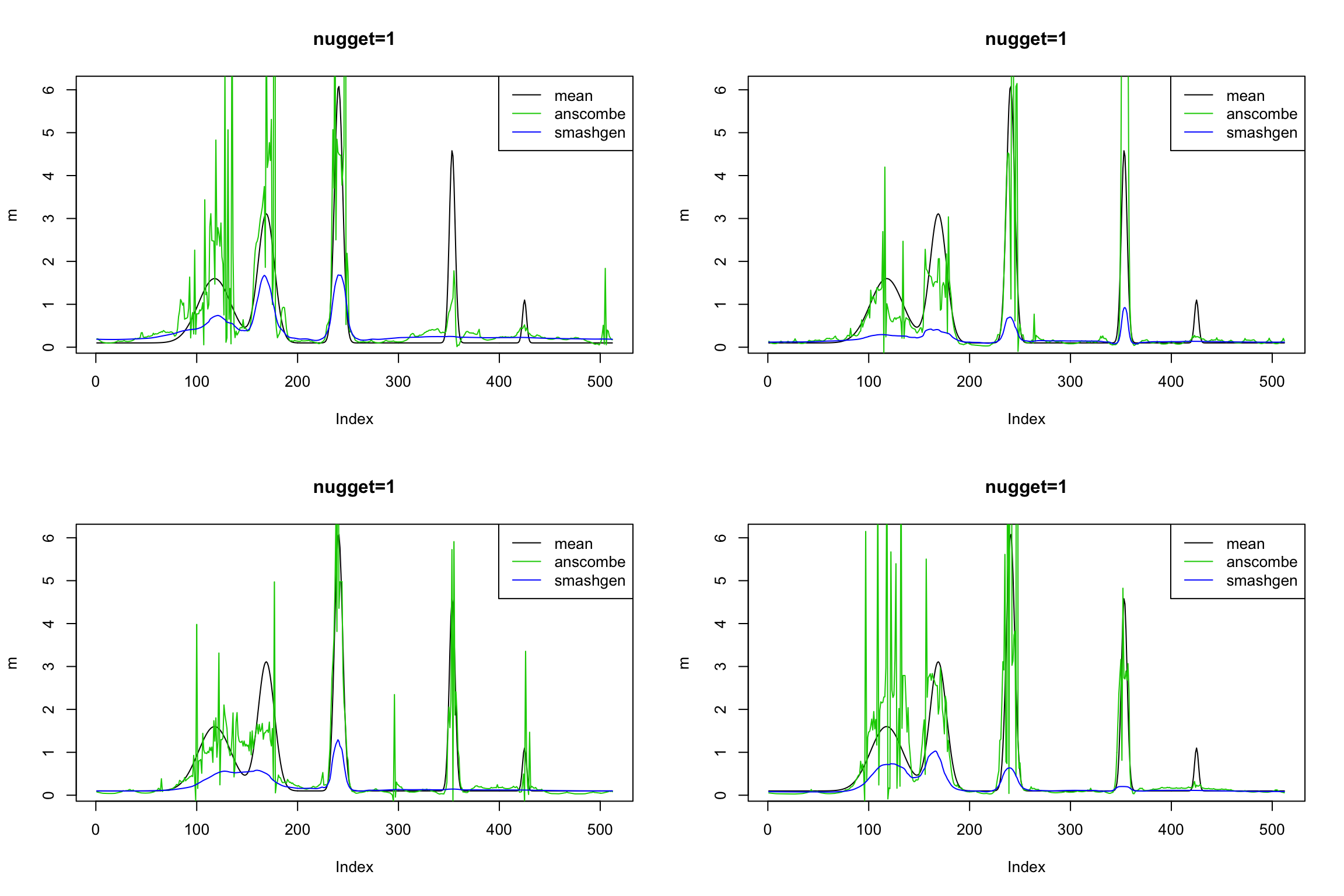
result=simu_study(m,sig=1)


mses=lapply(result, function(x){apply(x, 1, function(y){mean((y-m)^2)})})

#unlist(lapply(mses, mean))

par(mfrow=c(2,2))
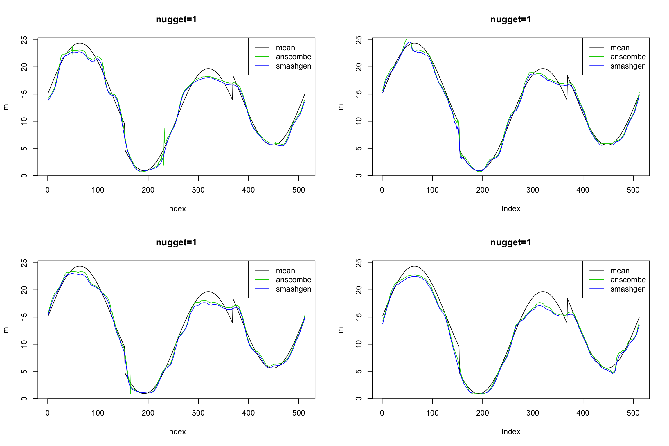
for (j in 1:4) {
  plot(m,type='l',main='nugget=1')
#lines(result$sr[1,],col=2)
lines(result$an[j,],col=3)
lines(result$ashp[j,],col=4)
legend('topright',c('mean','anscombe','smashgen'),lty=c(1,1,1),col=c(1,3,4))
#legend('topright',c('mean','square root','anscombe','smashgen'),lty=c(1,1,1,1),col=c(1,2,3,4))

}

Past versions of unnamed-chunk-7-1.png

Version	Author	Date
7386626	Dongyue Xie	2018-10-23

boxplot(mses,names = c('square root','anscombe','smashgen'),main='nugget=1',ylab='MSE')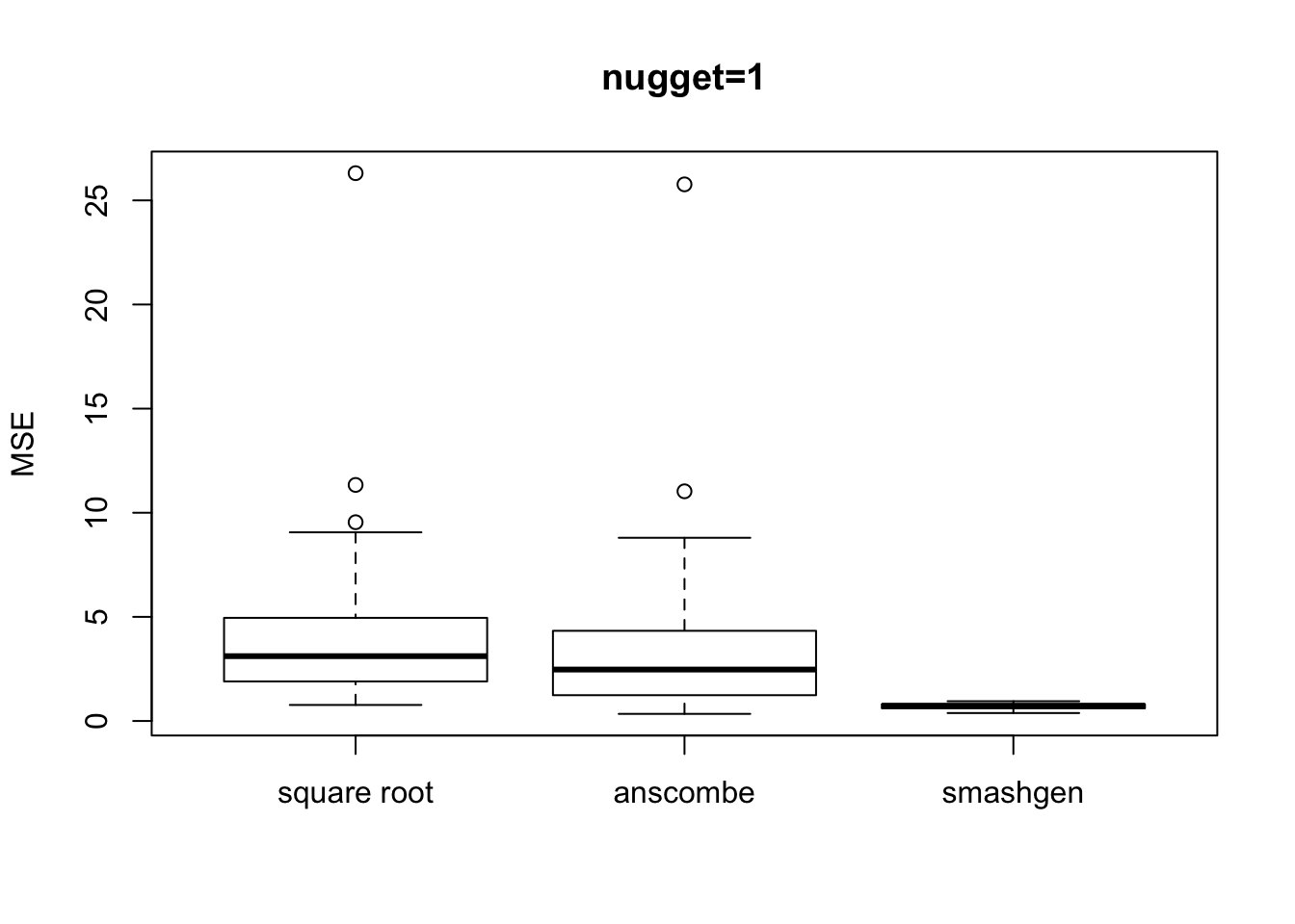

Past versions of unnamed-chunk-8-1.png

Version	Author	Date
7386626	Dongyue Xie	2018-10-23

###############

m=m*20+30
range(m)

[1]  32.0000 151.5263

result=simu_study(m)

mses=lapply(result, function(x){apply(x, 1, function(y){mean((y-m)^2)})})

#unlist(lapply(mses, mean))

par(mfrow=c(2,2))

for (j in 1:4) {
  plot(m,type='l',main='nugget=0')
lines(result$sr[j,],col=2)
lines(result$an[j,],col=3)
lines(result$ashp[j,],col=4)
legend('topright',c('mean','square root','anscombe','smashgen'),lty=c(1,1,1,1),col=c(1,2,3,4))

}

Past versions of unnamed-chunk-9-1.png

Version	Author	Date
7386626	Dongyue Xie	2018-10-23

boxplot(mses,names = c('square root','anscombe','smashgen'),main='nugget=0',ylab='MSE')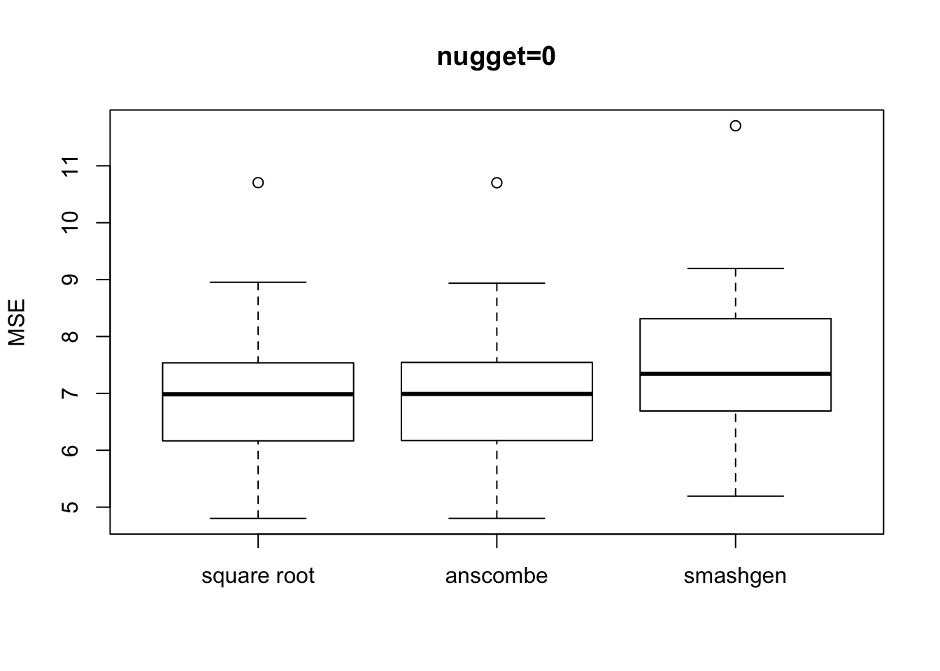

Past versions of unnamed-chunk-10-1.png

Version	Author	Date
7386626	Dongyue Xie	2018-10-23

Step function

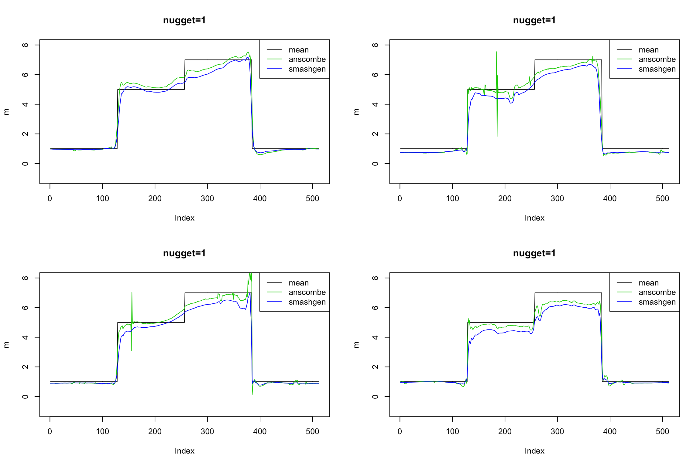
mean: (1,7)

m=c(rep(1,n/4),rep(5,n/4),rep(7,n/4),rep(1,n/4))

result=simu_study(m)

mses=lapply(result, function(x){apply(x, 1, function(y){mean((y-m)^2)})})

#unlist(lapply(mses, mean))

par(mfrow=c(2,2))

for (j in 1:4) {
  plot(m,type='l',main='nugget=1',ylim=c(-1,8))
#lines(result$sr[1,],col=2)
lines(result$an[j,],col=3)
lines(result$ashp[j,],col=4)
legend('topright',c('mean','anscombe','smashgen'),lty=c(1,1,1),col=c(1,3,4))
#legend('topright',c('mean','square root','anscombe','smashgen'),lty=c(1,1,1,1),col=c(1,2,3,4))

}

Past versions of unnamed-chunk-11-1.png

Version	Author	Date
7386626	Dongyue Xie	2018-10-23

boxplot(mses,names = c('square root','anscombe','smashgen'),main='nugget=0',ylab='MSE')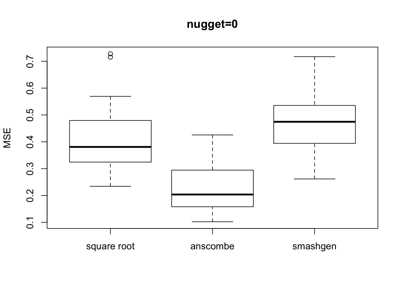

Past versions of unnamed-chunk-12-1.png

Version	Author	Date
7386626	Dongyue Xie	2018-10-23

Heavi Sine function

mean: (1,24)

m=wavethresh::DJ.EX(n)
m=m$heavi+15
range(m)

[1]  0.8749178 24.4167215

result=simu_study(m)

mses=lapply(result, function(x){apply(x, 1, function(y){mean((y-m)^2)})})

#unlist(lapply(mses, mean))

par(mfrow=c(2,2))

for (j in 1:4) {
  plot(m,type='l',main='nugget=1')
#lines(result$sr[1,],col=2)
lines(result$an[j,],col=3)
lines(result$ashp[j,],col=4)
legend('topright',c('mean','anscombe','smashgen'),lty=c(1,1,1),col=c(1,3,4))
#legend('topright',c('mean','square root','anscombe','smashgen'),lty=c(1,1,1,1),col=c(1,2,3,4))

}

Past versions of unnamed-chunk-13-1.png

Version	Author	Date
7386626	Dongyue Xie	2018-10-23

boxplot(mses,names = c('square root','anscombe','smashgen'),main='nugget=0',ylab='MSE')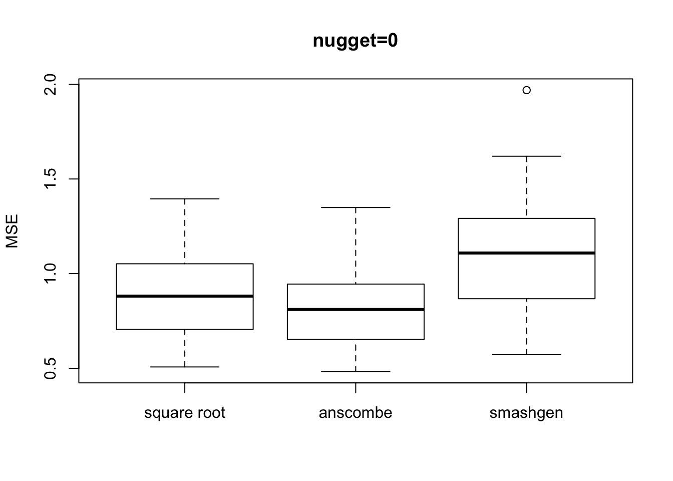

Session information

sessionInfo()

R version 3.6.1 (2019-07-05)
Platform: x86_64-apple-darwin15.6.0 (64-bit)
Running under: macOS High Sierra 10.13.6

Matrix products: default
BLAS:   /Library/Frameworks/R.framework/Versions/3.6/Resources/lib/libRblas.0.dylib
LAPACK: /Library/Frameworks/R.framework/Versions/3.6/Resources/lib/libRlapack.dylib

locale:
[1] en_US.UTF-8/en_US.UTF-8/en_US.UTF-8/C/en_US.UTF-8/en_US.UTF-8

attached base packages:
[1] stats     graphics  grDevices utils     datasets  methods   base     

other attached packages:
[1] smashrgen_0.1.2  wavethresh_4.6.8 MASS_7.3-51.4    caTools_1.17.1.2
[5] smashr_1.2-7     ashr_2.2-38     

loaded via a namespace (and not attached):
 [1] Rcpp_1.0.2        compiler_3.6.1    later_1.0.0      
 [4] git2r_0.26.1      workflowr_1.5.0   bitops_1.0-6     
 [7] iterators_1.0.12  tools_3.6.1       digest_0.6.21    
[10] evaluate_0.14     lattice_0.20-38   rlang_0.4.5      
[13] Matrix_1.2-17     foreach_1.4.7     yaml_2.2.0       
[16] parallel_3.6.1    xfun_0.10         stringr_1.4.0    
[19] knitr_1.25        fs_1.3.1          rprojroot_1.3-2  
[22] grid_3.6.1        data.table_1.12.6 glue_1.3.1       
[25] R6_2.4.0          rmarkdown_1.16    mixsqp_0.1-97    
[28] magrittr_1.5      whisker_0.4       backports_1.1.5  
[31] promises_1.1.0    codetools_0.2-16  htmltools_0.4.0  
[34] httpuv_1.5.2      stringi_1.4.3     doParallel_1.0.15
[37] pscl_1.5.2        truncnorm_1.0-8   SQUAREM_2017.10-1