Iterative vst

Smoothing exp family data

Observations are \(x\) count data which are modeled using Poisson distribution. Assume \(X\sim Pois(\mu)\), and \(\mu\) is smooth or ‘noisy’ smooth. Noisy smooth means \(\mu\) is conraminated by noise. We model it as \(\mu=h(m+\epsilon)\), where \(\epsilon\) is a random error \(\epsilon\sim N(0,\sigma^2)\) and \(h(\cdot)\) is a one-to-one continuous real valued function. The question is how to recover the smooth structure in \(\mu\).

Variance stabilizing transformation approach:

Derivation of anscombe transformation:

suppose \(X\sim Pois(\mu)\) and define \(t=X-\mu\), \(m=\mu+c\). Expand \(Y=\sqrt{X+c}=\sqrt{m+t}\) around \(t=0\) we have \(Y=m^{1/2}+\frac{1}{2}m^{-1/2}t-\frac{1}{8}m^{-3/2}t^2+\frac{1}{16}m^{-5/2}t^3+O(t^4)\).

Moments of \(t\): \(E(t)=0\), \(E(t^2)=\mu\), \(E(t^3)=\mu\), \(E(t^4)=3\mu^2+\mu\), \(E(t^6)=-\mu^4+15\mu^3+25\mu^2+\mu\)

Then the variance of \(Y\) is(using up to \(t^2\)) \(Var(Y)=\frac{1}{4}m^{-1}\mu+\frac{1}{64}m^{-3}(2\mu^2+\mu)-\frac{1}{8}m^{-2}\mu\) and if \(\mu\to\infty\), \(Var(Y)\to 1/4\).

How did Anscombe make \(c\) in nominator??? I think is to use higher order of t and let \(\mu\to\infty\).

\(Y=\sqrt{X+c}\) where \(c\) is a constant, \(c\geq 0\) and then \(Y\sim N(\sqrt{\mu+c},1/4)\) for large \(\mu\). (\(\mu\geq 4\) is already very good approx; \(\mu\geq 2\) is ok.) We can write \(Y=\sqrt{\mu+c}+N(0,1/4)\) and so \(Y=m+\epsilon+N(0,1/4)\). If \(\sigma^2\) is known, we can apply any Gaussian non-parametric smoothing methods to estiamte \(m\); if unkown, we might want to estiamte \(\sigma^2\) or \(\sigma^2+1/4\) first.

One problem is that \(Var(Y)\approx 1/4\) only holds for large enough \(\mu\) and what if we have observations like \(x=0\). One immidiate strategy is to use 0 variance for 0 \(x\). But the probability of observing \(x=0\) when \(\mu=1,2\) is 0.37, 0.14 respectively. So we may ask if there are better way to do this.

dpois(0,1)

[1] 0.3678794

dpois(0,2)

[1] 0.1353353

dpois(0,3)

[1] 0.04978707

One way is to approximate the variance using \(\mu\). Then we need a formula bwt var and mean. From the plot below, the simulated variance line is from \(10^5\) ramdom samples so it can be regared as the ‘true’ variance of \(Y=\sqrt{X+3/8}\); formula in anscombe’s paper is obtained when \(\mu\to\infty\) so it cannot deal with small mean; using 2nd order taylor series expnasion always under-estimate the variance. So we might need higher order approximation but it’s much more complicated.

# mu=1
c=3/8
# m=mu+c
# t=seq(-m,m,length.out = 1000)
# plot(t,sqrt(t+m),type='l')
# #taylor series expnasion around t=0
# taylor=sqrt(m)+1/sqrt(m)*t/2-m^(-1.5)/8*t^2+m^(-2.5)/16*t^3
# lines(t,taylor,col=4)

mu=seq(0,10,length.out = 1000)
m=mu+c
var.y=mu/(4*m)+(2*mu^2+mu)/(64*m^3)-mu/(8*m^2)
var.ans=1/4*(1+(32*c^2-52*c+17)/(32*mu^2))

var.sim=c()
set.seed(12345)
for (i  in 1:length(mu)) {
  x=rpois(1e6,mu[i])
  var.sim[i]=var(sqrt(x+3/8))
}

plot(mu,var.y,type='l',ylim=c(0,0.5))
lines(mu,var.sim,col=3)
lines(mu,var.ans,col=4)
abline(a=0.25,b=0,lty=2)
legend('bottomright',c('anscombe formula','2nd order taylor','simulated'),col=c(4,1,3),lty=c(1,1,1))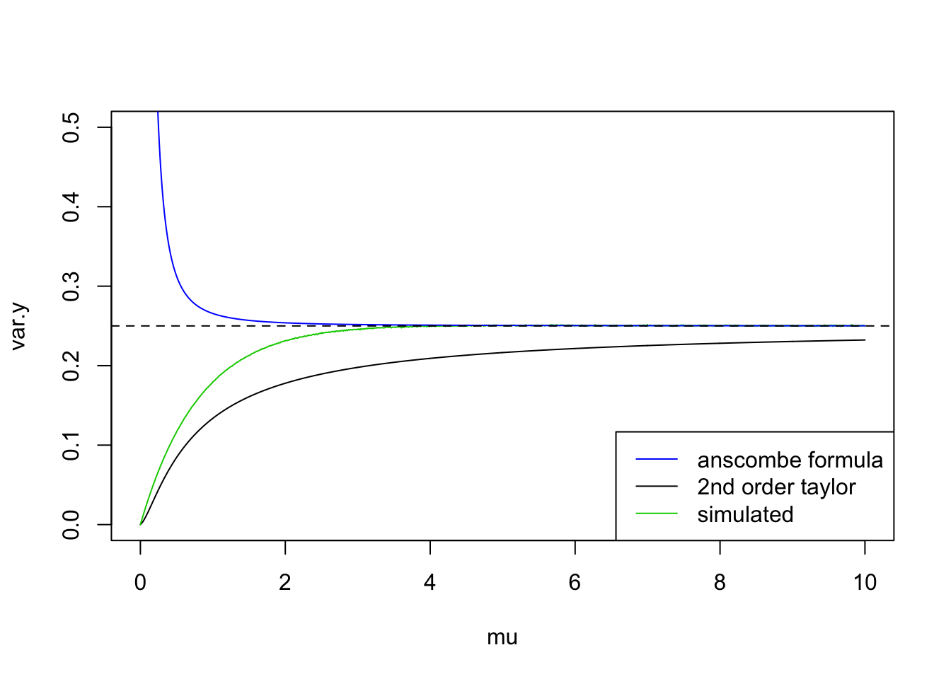

Functional mixed models

A good tutorial on functional data analysis.

shim&stephens:

This is a ‘Function on scalar regression’ case: response(count) is functional data and covariate(genotype) is a scalar. For each subject \(i=1,...,n\), \(y_i(s)=x_i^T\beta(s)+\epsilon_i(s)\), where \(s\) is the grid of time points, \(|s|=T\) the total length of observations of subject \(i\). For example, if \(x_i=(1,x_{i1})\), then \(y_i(s)=\beta_0(s)+x_{i1}\beta_1(s)+\epsilon_i(s)\). So \(\beta_0(s)\) is global mean function of all subjects and \(\beta_1(s)\) is global coefficients function of all subjects. We can write the model as \(Y=XB+E\) where \(T\in R^{n*T}\), \(X\in R^{n*p}\), \(B\in R^{p*T}\) and \(E\) is n by T error matrix.

So the idea for dealing with data in shim and stephens, taking transformation and nugget effect into consideration is:

suppose we observe a sequence of \(x\) from an exponential family distribution, we do a transformation on X and obtain \(y=h(x)=m+\beta z+\epsilon_1+\epsilon_2\) where \(m\) has a smooth structure, \(\epsilon\)s are normal distributed random errors. Then apply DWT to \(y\) yeild \(Wy=Wm+W\beta z+W\epsilon_1+W\epsilon_2\). Then we can use similar methods in paper to do inference. A problem is how to estimate nugget effect.

Session information

sessionInfo()

R version 3.5.1 (2018-07-02)
Platform: x86_64-apple-darwin15.6.0 (64-bit)
Running under: macOS High Sierra 10.13.6

Matrix products: default
BLAS: /Library/Frameworks/R.framework/Versions/3.5/Resources/lib/libRblas.0.dylib
LAPACK: /Library/Frameworks/R.framework/Versions/3.5/Resources/lib/libRlapack.dylib

locale:
[1] en_US.UTF-8/en_US.UTF-8/en_US.UTF-8/C/en_US.UTF-8/en_US.UTF-8

attached base packages:
[1] stats     graphics  grDevices utils     datasets  methods   base     

loaded via a namespace (and not attached):
 [1] workflowr_1.1.1   Rcpp_0.12.18      digest_0.6.17    
 [4] rprojroot_1.3-2   R.methodsS3_1.7.1 backports_1.1.2  
 [7] git2r_0.23.0      magrittr_1.5      evaluate_0.11    
[10] stringi_1.2.4     whisker_0.3-2     R.oo_1.22.0      
[13] R.utils_2.7.0     rmarkdown_1.10    tools_3.5.1      
[16] stringr_1.3.1     yaml_2.2.0        compiler_3.5.1   
[19] htmltools_0.3.6   knitr_1.20