Poisson sequence with Spike mean
Dongyue Xie
May 21, 2018
Last updated: 2018-05-24
workflowr checks: (Click a bullet for more information)-
✔ R Markdown file: up-to-date
Great! Since the R Markdown file has been committed to the Git repository, you know the exact version of the code that produced these results.
-
✔ Environment: empty
Great job! The global environment was empty. Objects defined in the global environment can affect the analysis in your R Markdown file in unknown ways. For reproduciblity it’s best to always run the code in an empty environment.
-
✔ Seed:
set.seed(20180501)The command
set.seed(20180501)was run prior to running the code in the R Markdown file. Setting a seed ensures that any results that rely on randomness, e.g. subsampling or permutations, are reproducible. -
✔ Session information: recorded
Great job! Recording the operating system, R version, and package versions is critical for reproducibility.
-
Great! You are using Git for version control. Tracking code development and connecting the code version to the results is critical for reproducibility. The version displayed above was the version of the Git repository at the time these results were generated.✔ Repository version: f3f3fbf
Note that you need to be careful to ensure that all relevant files for the analysis have been committed to Git prior to generating the results (you can usewflow_publishorwflow_git_commit). workflowr only checks the R Markdown file, but you know if there are other scripts or data files that it depends on. Below is the status of the Git repository when the results were generated:
Note that any generated files, e.g. HTML, png, CSS, etc., are not included in this status report because it is ok for generated content to have uncommitted changes.Ignored files: Ignored: .Rhistory Ignored: .Rproj.user/ Ignored: log/ Untracked files: Untracked: analysis/binom.Rmd Untracked: analysis/covariate.Rmd Untracked: analysis/glm.Rmd Untracked: analysis/overdis.Rmd Untracked: analysis/smashtutorial.Rmd Untracked: analysis/test.Rmd Untracked: data/treas_bill.csv Untracked: docs/figure/smashtutorial.Rmd/ Untracked: docs/figure/test.Rmd/ Unstaged changes: Modified: analysis/ashpmean.Rmd Modified: analysis/nugget.Rmd
Expand here to see past versions:
From the Poisson sequence with unknown variance simulations, we notice that 1. smashgen performs poorly when the mean function has sudden changes like spikes; 2. smashgen is not as good as smash.pois sometimes when \(\sigma\) is small and the range of mean function is small.
The performance of smashgen is worse than smash.pois for spike mean, especialy when the range of \(\mu\) is small. Smashgen cannot capture the spikes properly which results in huge squared errors. The smash.pois could capture the spikes and it gives noisy fit for the low mean area so it’s MSE is much smaller. Let’s figure out the reason.
One possible reason that causes the issue is that smashgen gives very large fit to the spikes.
Plots of smashgen smoothed wavelets. Blue curves are from smashgen and the black ones are truth.
library(smashrgen)
spike.f = function(x) (0.75 * exp(-500 * (x - 0.23)^2) + 1.5 * exp(-2000 * (x - 0.33)^2) + 3 * exp(-8000 * (x - 0.47)^2) + 2.25 * exp(-16000 *
    (x - 0.69)^2) + 0.5 * exp(-32000 * (x - 0.83)^2))
n = 256
t = 1:n/n
m = spike.f(t)

m=m*2+0.1
range(m)
[1] 0.100000 6.025467m=log(m)
sigma=0.1
set.seed(12345)
lamda=exp(m+rnorm(length(m),0,sigma))
x=rpois(length(m),lamda)
x.fit=smash_gen(x)
plot(x,col='gray80',main='sigma=0.1')
lines(exp(m))
lines(x.fit,col=4)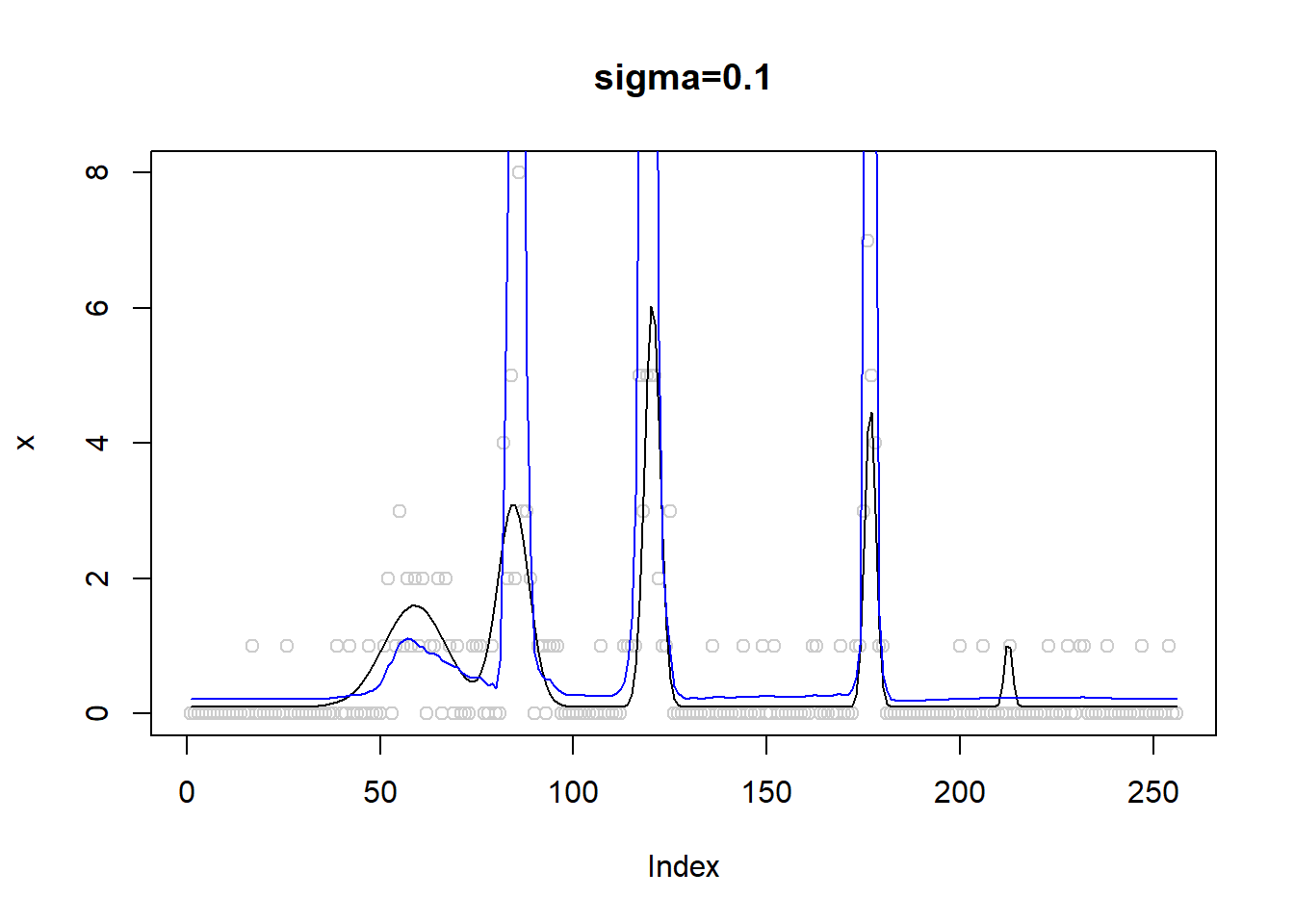
Expand here to see past versions of unnamed-chunk-1-1.png:
| Version | Author | Date |
|---|---|---|
| 0df1e15 | Dongyue | 2018-05-21 |
To figure out the reason, we make the following plot.
x.ash=ash(rep(0,n),1,lik=lik_pois(x))$result$PosteriorMean
y=log(x.ash)+(x-x.ash)/x.ash
plot(x,col='gray80',ylim = c(-2,10))
lines(exp(m))
lines(x.ash,col=4)
lines(y,col=3,type = 'p',pch=1)
lines(m,col=2)
lines(log(x.fit),col=2,lty=2)
legend('topright',
       c('data','true mean','ash shrinked','normal approx data','true normal mean','smashgen normal mean'),
       lty=c(0,1,1,0,1,2),
       pch=c(1,NA,NA,1,NA,NA),

       cex=1,col=c('gray80',1,4,3,2,2))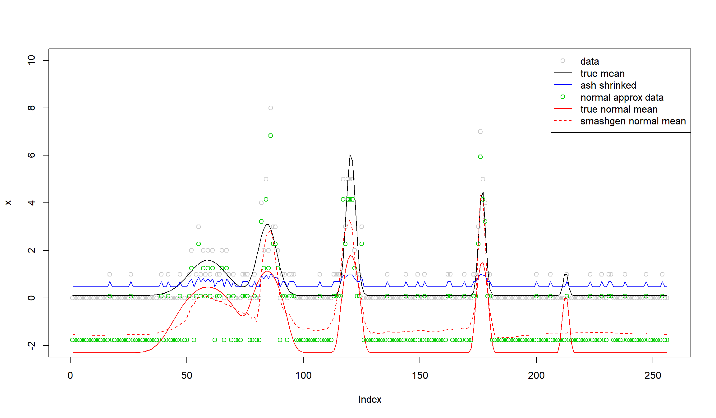
Expand here to see past versions of unnamed-chunk-2-1.png:
| Version | Author | Date |
|---|---|---|
| 0df1e15 | Dongyue | 2018-05-21 |
\(\sigma=1\)
sigma=1
set.seed(12345)
lamda=exp(m+rnorm(length(m),0,sigma))
x=rpois(length(m),lamda)
x.fit=smash_gen(x)
plot(x,col='gray80',main='sigma=1')
lines(exp(m))
lines(x.fit,col=4)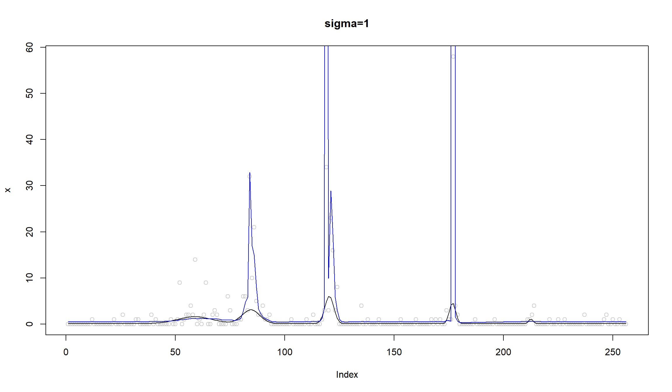
Expand here to see past versions of unnamed-chunk-3-1.png:
| Version | Author | Date |
|---|---|---|
| 0df1e15 | Dongyue | 2018-05-21 |
x.ash=ash(rep(0,n),1,lik=lik_pois(x))$result$PosteriorMean
y=log(x.ash)+(x-x.ash)/x.ash
plot(x,col='gray80',ylim = c(-2,10))
lines(exp(m))
lines(x.ash,col=4)
lines(y,col=3,type = 'p',pch=1)
lines(m,col=2)
lines(log(x.fit),col=2,lty=2)
legend('topright',
       c('data','true mean','ash shrinked','normal approx data','true normal mean','est normal mean'),
       lty=c(0,1,1,0,1,2),
       pch=c(1,NA,NA,1,NA,NA),

       cex=1,col=c('gray80',1,4,3,2,2))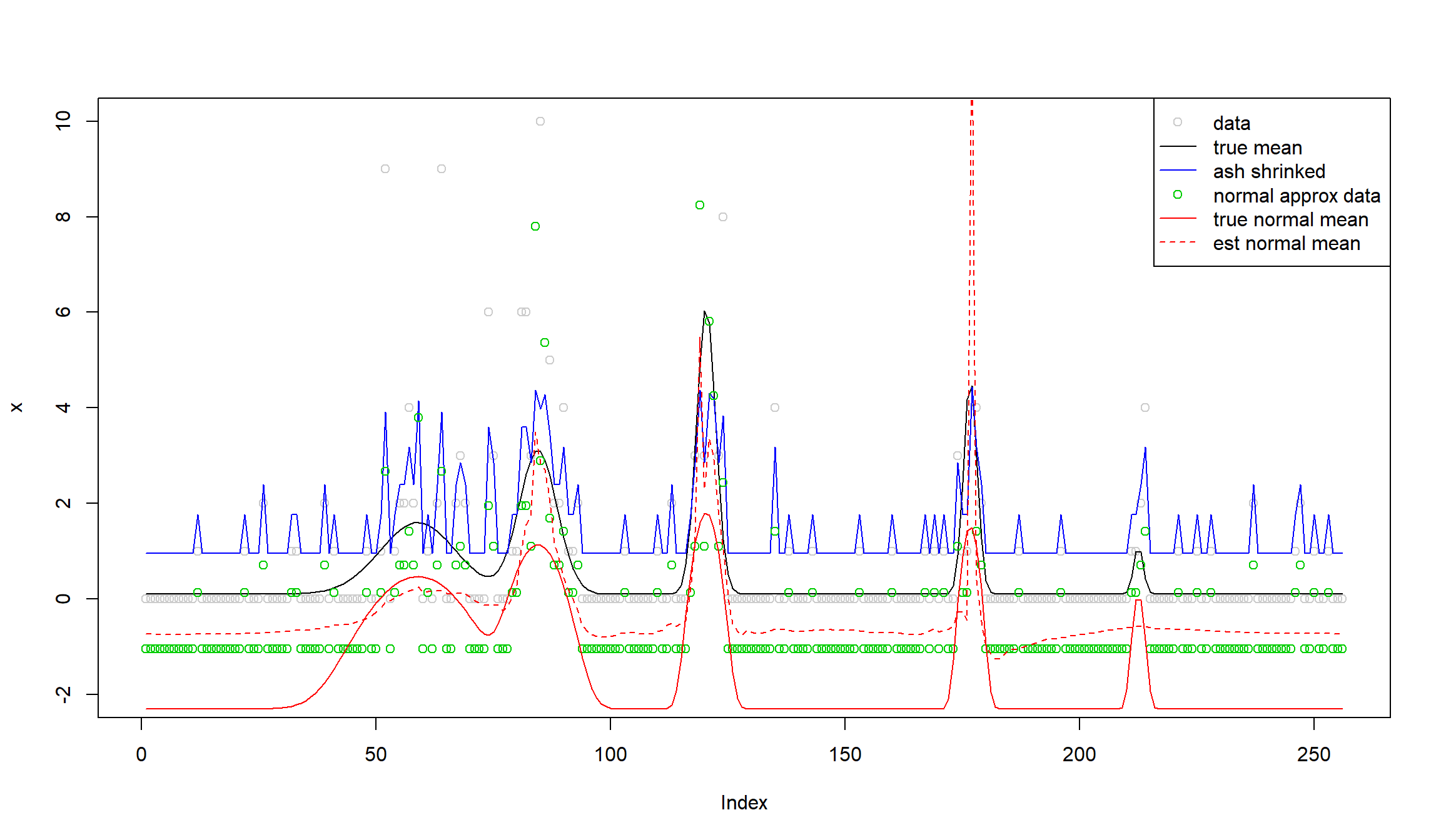
Expand here to see past versions of unnamed-chunk-3-2.png:
| Version | Author | Date |
|---|---|---|
| 0df1e15 | Dongyue | 2018-05-21 |
If we use the robust version:
par(mfrow=c(1,2))
sigma=0.1
set.seed(12345)
lamda=exp(m+rnorm(length(m),0,sigma))
x=rpois(length(m),lamda)
x.fit=smash_gen(x,robust = T)
plot(x,col='gray80',main='sigma=0.1')
lines(exp(m))
lines(x.fit,col=4)
sigma=1
set.seed(12345)
lamda=exp(m+rnorm(length(m),0,sigma))
x=rpois(length(m),lamda)
x.fit=smash_gen(x,robust = T)
plot(x,col='gray80',main='simga=1')
lines(exp(m))
lines(x.fit,col=4)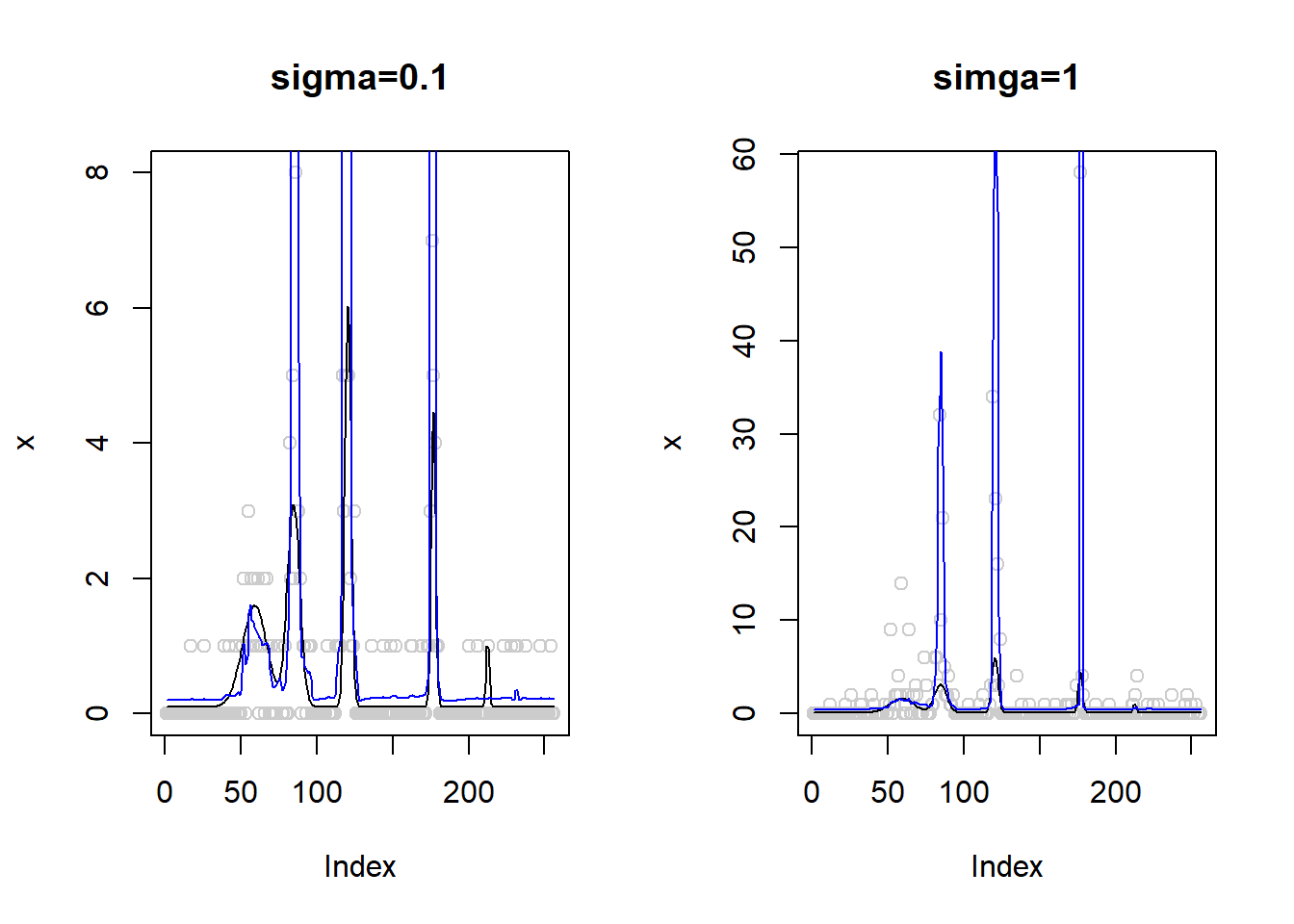
Expand here to see past versions of unnamed-chunk-4-1.png:
| Version | Author | Date |
|---|---|---|
| 0df1e15 | Dongyue | 2018-05-21 |
It does not help for now.
It seems that ash shrinks the data to the mean too much such that the normal approximated data consistently larger than what we want.
If we don’t use the ash shinkage and use more iterations:
par(mfrow=c(1,2))
sigma=0.1
set.seed(12345)
lamda=exp(m+rnorm(length(m),0,sigma))
x=rpois(length(m),lamda)
x.fit=smash_gen(x,robust = T,ashp = F,niter=20,verbose = T)
plot(x,col='gray80',main='sigma=0.1')
lines(exp(m))
lines(x.fit,col=4)
sigma=1
set.seed(12345)
lamda=exp(m+rnorm(length(m),0,sigma))
x=rpois(length(m),lamda)
x.fit=smash_gen(x,robust = T,ashp = F,niter=20,verbose = T)
plot(x,col='gray80',main='simga=1')
lines(exp(m))
lines(x.fit,col=4)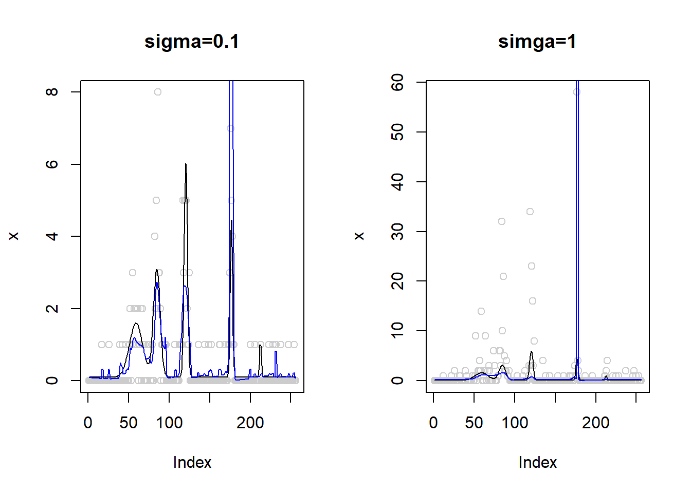
Expand here to see past versions of unnamed-chunk-5-1.png:
| Version | Author | Date |
|---|---|---|
| 0df1e15 | Dongyue | 2018-05-21 |
Still, the algorithm does not converge so we still see the huge spike on the plot.
Signal to noise ratio is too high!
When the range of mean function is around \((0.1,6)\), the signal to noise ratio is too high.
par(mfrow=c(1,2))
plot(1/exp(m)+0.1,type='l',col=4,ylim=c(0,11),main='sigma=0.1',ylab='variance')
lines(rep(var(m),n),type='l')
legend('bottomright',c('noise','signal'),lty=c(1,1),col=c(4,1))
plot(1/exp(m)+1,type='l',col=4,ylim=c(0,11),main='sigma=1',ylab='variance')
lines(rep(var(m),n),type='l')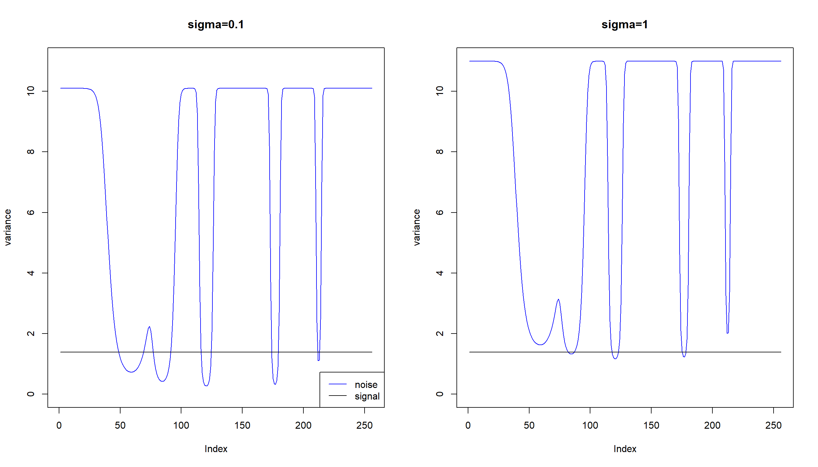
Expand here to see past versions of unnamed-chunk-6-1.png:
| Version | Author | Date |
|---|---|---|
| 0df1e15 | Dongyue | 2018-05-21 |
#legend('bottomright',c('noise','signal'),lty=c(1,1),col=c(4,1))If we choose \(\mu\) in around \((0.1,60)\):
m = spike.f(t)

m=m*20+0.1
m=log(m)
range(exp(m))
[1] 0.10000 59.35467par(mfrow=c(1,2))
plot(1/exp(m)+0.1,type='l',col=4,ylim=c(0,11),main='sigma=0.1',ylab='variance')
lines(rep(var(m),n),type='l')
legend('bottomright',c('noise','signal'),lty=c(1,1),col=c(4,1))
plot(1/exp(m)+1,type='l',col=4,ylim=c(0,11),main='sigma=1',ylab='variance')
lines(rep(var(m),n),type='l')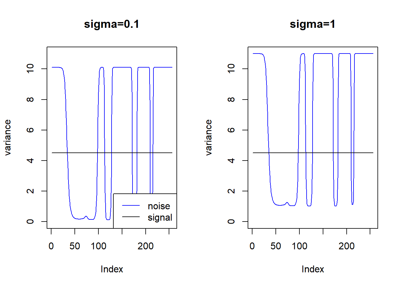
Expand here to see past versions of unnamed-chunk-7-1.png:
| Version | Author | Date |
|---|---|---|
| 0df1e15 | Dongyue | 2018-05-21 |
Then the ‘spike’ issue disappears:
par(mfrow=c(1,2))
sigma=0.1
set.seed(12345)
lamda=exp(m+rnorm(length(m),0,sigma))
x=rpois(length(m),lamda)
x.fit=smash_gen(x,robust = T)
plot(x,col='gray80',main='sigma=0.1')
lines(exp(m))
lines(x.fit,col=4)
sigma=1
set.seed(12345)
lamda=exp(m+rnorm(length(m),0,sigma))
x=rpois(length(m),lamda)
x.fit=smash_gen(x,robust = T)
plot(x,col='gray80',main='simga=1')
lines(exp(m))
lines(x.fit,col=4)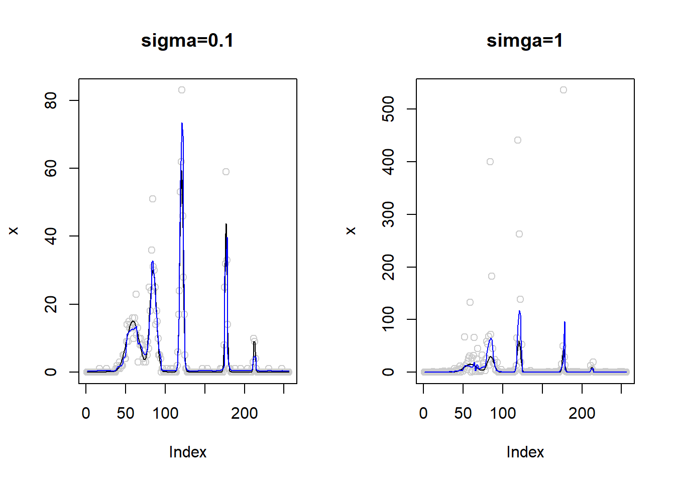
Expand here to see past versions of unnamed-chunk-8-1.png:
| Version | Author | Date |
|---|---|---|
| 0df1e15 | Dongyue | 2018-05-21 |
Increase ‘sample size’!
m = spike.f(t)

m=m*100+100
m=log(m)
range(exp(m))
[1] 100.0000 396.2733par(mfrow=c(1,2))
plot(1/exp(m)+0.1,type='l',col=4,ylim=c(0,11),main='sigma=0.1',ylab='variance')
lines(rep(var(m),n),type='l')
legend('bottomright',c('noise','signal'),lty=c(1,1),col=c(4,1))
plot(1/exp(m)+1,type='l',col=4,ylim=c(0,11),main='sigma=1',ylab='variance')
lines(rep(var(m),n),type='l')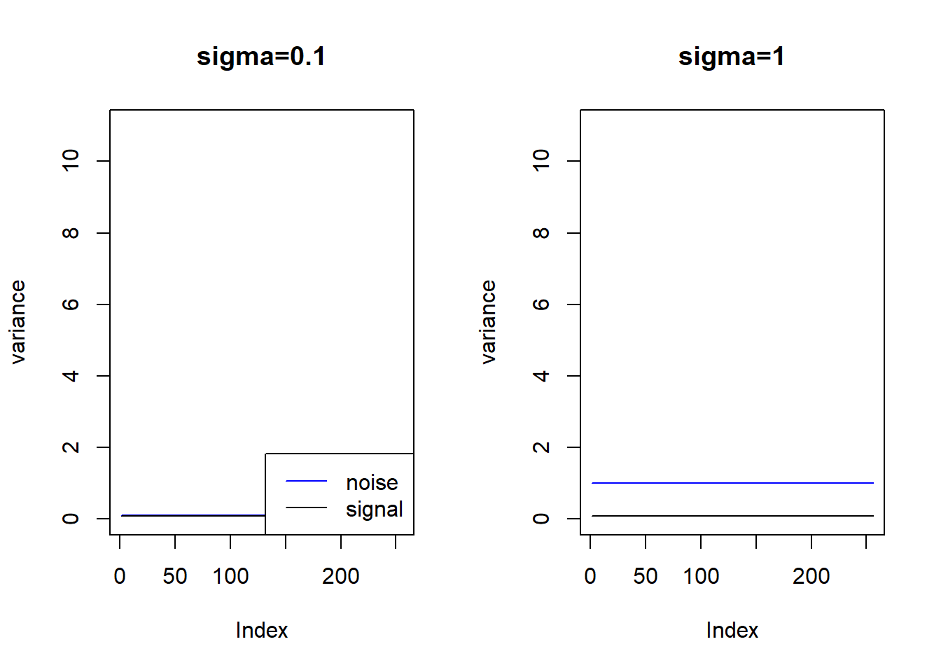
par(mfrow=c(1,2))
sigma=0.1
set.seed(12345)
lamda=exp(m+rnorm(length(m),0,sigma))
x=rpois(length(m),lamda)
x.fit=smash_gen(x,robust = T)
plot(x,col='gray80',main='sigma=0.1')
lines(exp(m))
lines(x.fit,col=4)
sigma=1
set.seed(12345)
lamda=exp(m+rnorm(length(m),0,sigma))
x=rpois(length(m),lamda)
x.fit=smash_gen(x,robust = T)
plot(x,col='gray80',main='simga=1')
lines(exp(m))
lines(x.fit,col=4)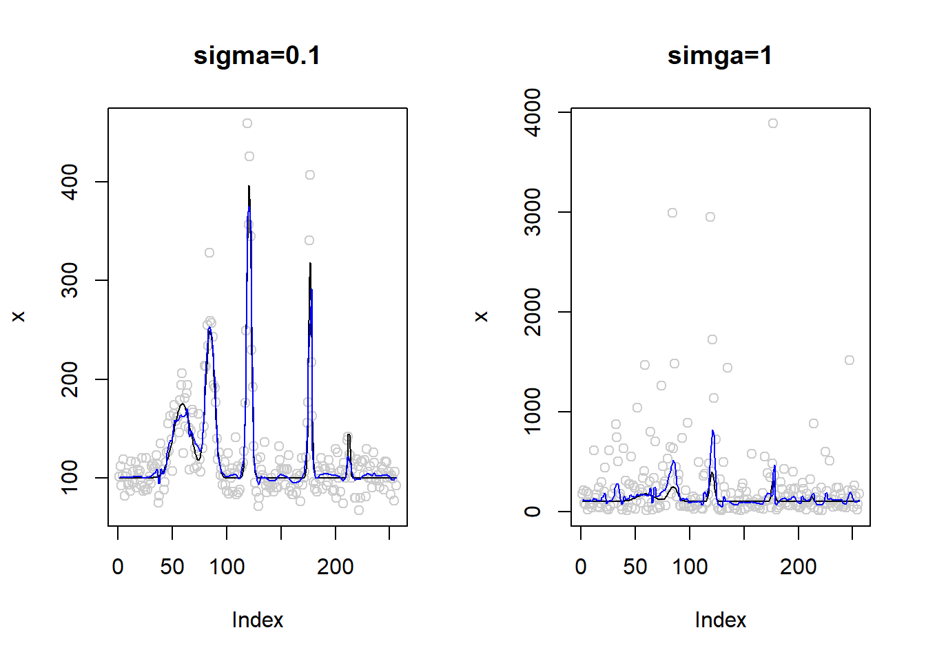
Session information
sessionInfo()R version 3.4.0 (2017-04-21)
Platform: x86_64-w64-mingw32/x64 (64-bit)
Running under: Windows 10 x64 (build 16299)
Matrix products: default
locale:
[1] LC_COLLATE=English_United States.1252
[2] LC_CTYPE=English_United States.1252
[3] LC_MONETARY=English_United States.1252
[4] LC_NUMERIC=C
[5] LC_TIME=English_United States.1252
attached base packages:
[1] stats graphics grDevices utils datasets methods base
other attached packages:
[1] smashrgen_0.1.0 wavethresh_4.6.8 MASS_7.3-47 caTools_1.17.1
[5] ashr_2.2-7 smashr_1.1-5
loaded via a namespace (and not attached):
[1] Rcpp_0.12.16 compiler_3.4.0 git2r_0.21.0
[4] workflowr_1.0.1 R.methodsS3_1.7.1 R.utils_2.6.0
[7] bitops_1.0-6 iterators_1.0.8 tools_3.4.0
[10] digest_0.6.13 evaluate_0.10 lattice_0.20-35
[13] Matrix_1.2-9 foreach_1.4.3 yaml_2.1.19
[16] parallel_3.4.0 stringr_1.3.0 knitr_1.20
[19] REBayes_1.3 rprojroot_1.3-2 grid_3.4.0
[22] data.table_1.10.4-3 rmarkdown_1.8 magrittr_1.5
[25] whisker_0.3-2 backports_1.0.5 codetools_0.2-15
[28] htmltools_0.3.5 assertthat_0.2.0 stringi_1.1.6
[31] Rmosek_8.0.69 doParallel_1.0.11 pscl_1.4.9
[34] truncnorm_1.0-7 SQUAREM_2017.10-1 R.oo_1.21.0 This reproducible R Markdown analysis was created with workflowr 1.0.1