Poisson nugget effect, unknown variance
Dongyue Xie
May 13, 2018
Last updated: 2018-05-21
workflowr checks: (Click a bullet for more information)-
✔ R Markdown file: up-to-date
Great! Since the R Markdown file has been committed to the Git repository, you know the exact version of the code that produced these results.
-
✔ Environment: empty
Great job! The global environment was empty. Objects defined in the global environment can affect the analysis in your R Markdown file in unknown ways. For reproduciblity it’s best to always run the code in an empty environment.
-
✔ Seed:
set.seed(20180501)The command
set.seed(20180501)was run prior to running the code in the R Markdown file. Setting a seed ensures that any results that rely on randomness, e.g. subsampling or permutations, are reproducible. -
✔ Session information: recorded
Great job! Recording the operating system, R version, and package versions is critical for reproducibility.
-
Great! You are using Git for version control. Tracking code development and connecting the code version to the results is critical for reproducibility. The version displayed above was the version of the Git repository at the time these results were generated.✔ Repository version: 341aecb
Note that you need to be careful to ensure that all relevant files for the analysis have been committed to Git prior to generating the results (you can usewflow_publishorwflow_git_commit). workflowr only checks the R Markdown file, but you know if there are other scripts or data files that it depends on. Below is the status of the Git repository when the results were generated:
Note that any generated files, e.g. HTML, png, CSS, etc., are not included in this status report because it is ok for generated content to have uncommitted changes.Ignored files: Ignored: .Rhistory Ignored: .Rproj.user/ Ignored: log/ Untracked files: Untracked: analysis/binom.Rmd Untracked: analysis/overdis.Rmd Untracked: analysis/smashtutorial.Rmd Untracked: analysis/test.Rmd Untracked: data/treas_bill.csv Untracked: docs/figure/smashtutorial.Rmd/ Untracked: docs/figure/test.Rmd/ Unstaged changes: Modified: analysis/ashpmean.Rmd Modified: analysis/nugget.Rmd
Expand here to see past versions:
| File | Version | Author | Date | Message |
|---|---|---|---|---|
| Rmd | 341aecb | Dongyue | 2018-05-21 | poi unknown version revise |
| Rmd | ca1e50a | Dongyue | 2018-05-21 | edit |
| Rmd | f7be0e4 | Dongyue | 2018-05-21 | edit |
| html | 594edf1 | Dongyue | 2018-05-17 | edit |
| Rmd | f7f7273 | Dongyue | 2018-05-16 | edit |
| Rmd | fc2c755 | Dongyue | 2018-05-16 | edit |
| Rmd | 996d337 | Dongyue | 2018-05-14 | poisson data unkown variance |
Simulations of Poisson nugget effect(unkown).
Previously, we have studies the methods to estimate unknown \(\sigma\) in the model \(Y_t=\mu_t+N(0,\sigma^2)+N(0,s_t^2)\). Here, we apply mle and smashu methods and compare them with smash as well as smashgen with known \(sigma\). The measure of accuracy is mean square error. Plots are also given as visual aid.
library(smashrgen)
library(ggplot2)
#' Simulation study comparing smash and smashgen
simu_study=function(m,sigma,nsimu=100,seed=12345,
niter=1,family='DaubExPhase',ashp=TRUE,verbose=FALSE,robust=FALSE,
tol=1e-2,return.x=F,filter.number=1){
set.seed(seed)
smash.err=c()
smashgen.err=c()
smashgen.smashu.err=c()
smashgen.mle.err=c()
x.data=c()
smashgen.smashu.out=c()
for(k in 1:nsimu){
lamda=exp(m+rnorm(length(m),0,sigma))
x=rpois(length(m),lamda)
x.data=rbind(x.data,x)
#fit data
smash.out=smash.poiss(x)
smashgen.out=smash_gen(x,dist_family = 'poisson',sigma = sigma,ashp=ashp,robust=robust,niter=niter,verbose = verbose,wave_family = family,filter.number = filter.number)
smashu.out=smash_gen(x,dist_family = 'poisson',y_var_est = 'smashu',ashp=ashp,robust=robust,niter=niter,verbose = verbose,wave_family = family,filter.number = filter.number)
smashgen.smashu.out=rbind(smashgen.smashu.out,smashu.out)
mle.out=smash_gen(x,dist_family = 'poisson',y_var_est = 'mle',
ashp=ashp,robust=robust,niter=niter,verbose = verbose,wave_family = family,filter.number = filter.number)
smash.err[k]=mse(exp(m),smash.out)
smashgen.err[k]=mse(exp(m),smashgen.out)
smashgen.smashu.err[k]=mse(exp(m),smashu.out)
smashgen.mle.err[k]=mse(exp(m),mle.out)
}
if(return.x){
return(list(est=list(smash.out=smash.out,smashgen.out=smashgen.out,smashu.out=smashu.out,mle.out=mle.out,x=x.data,smashgen.smashu.out=smashgen.smashu.out),err=data.frame(smash=smash.err,smashgen=smashgen.err,
smashgen.smashu=smashgen.smashu.err,smashgen.mle=smashgen.mle.err)))
}else{
return(list(est=list(smash.out=smash.out,smashgen.out=smashgen.out,smashu.out=smashu.out,mle.out=mle.out,x=x),err=data.frame(smash=smash.err,smashgen=smashgen.err,
smashgen.smashu=smashgen.smashu.err,smashgen.mle=smashgen.mle.err)))
}
}Simulation 1: Constant trend Poisson nugget
\(\sigma=0.1\)
m=rep(1,128)
result=simu_study(m,0.1)
par(mfrow=c(2,2))
plot(result$est$x,col='gray80',ylab='',main='smash')
lines(exp(m),col=1)
lines(result$est$smash.out,col=4)
plot(result$est$x,col='gray80',ylab='',main='smashgen: known sigma')
lines(exp(m),col=1)
lines(result$est$smashgen.out,col=4)
plot(result$est$x,col='gray80',ylab='',main='smashgen: (sigma^2+s_t^2) from smash')
lines(exp(m),col=1)
lines(result$est$smashu.out,col=4)
plot(result$est$x,col='gray80',ylab='',main='smashgen: sigma from mle')
lines(exp(m),col=1)
lines(result$est$mle.out,col=4)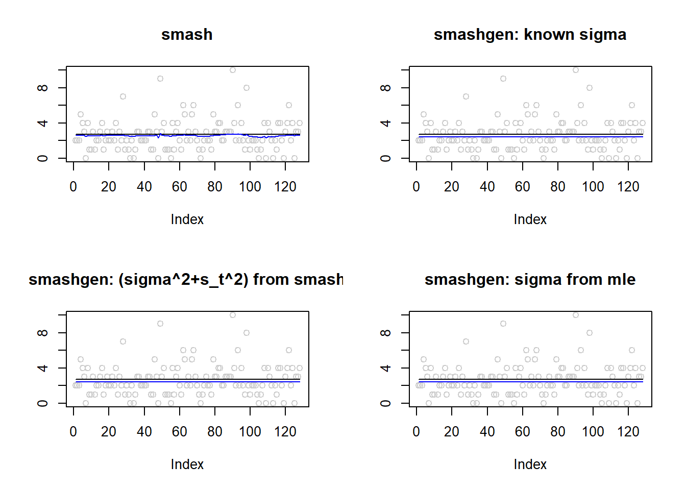
Expand here to see past versions of unnamed-chunk-3-1.png:
| Version | Author | Date |
|---|---|---|
| 594edf1 | Dongyue | 2018-05-17 |
round(apply(result$err,2,mean),4) smash smashgen smashgen.smashu smashgen.mle
0.0318 0.0299 0.0313 0.0299 ggplot(df2gg(result$err),aes(x=method,y=MSE))+geom_boxplot(aes(fill=method))+labs(x='')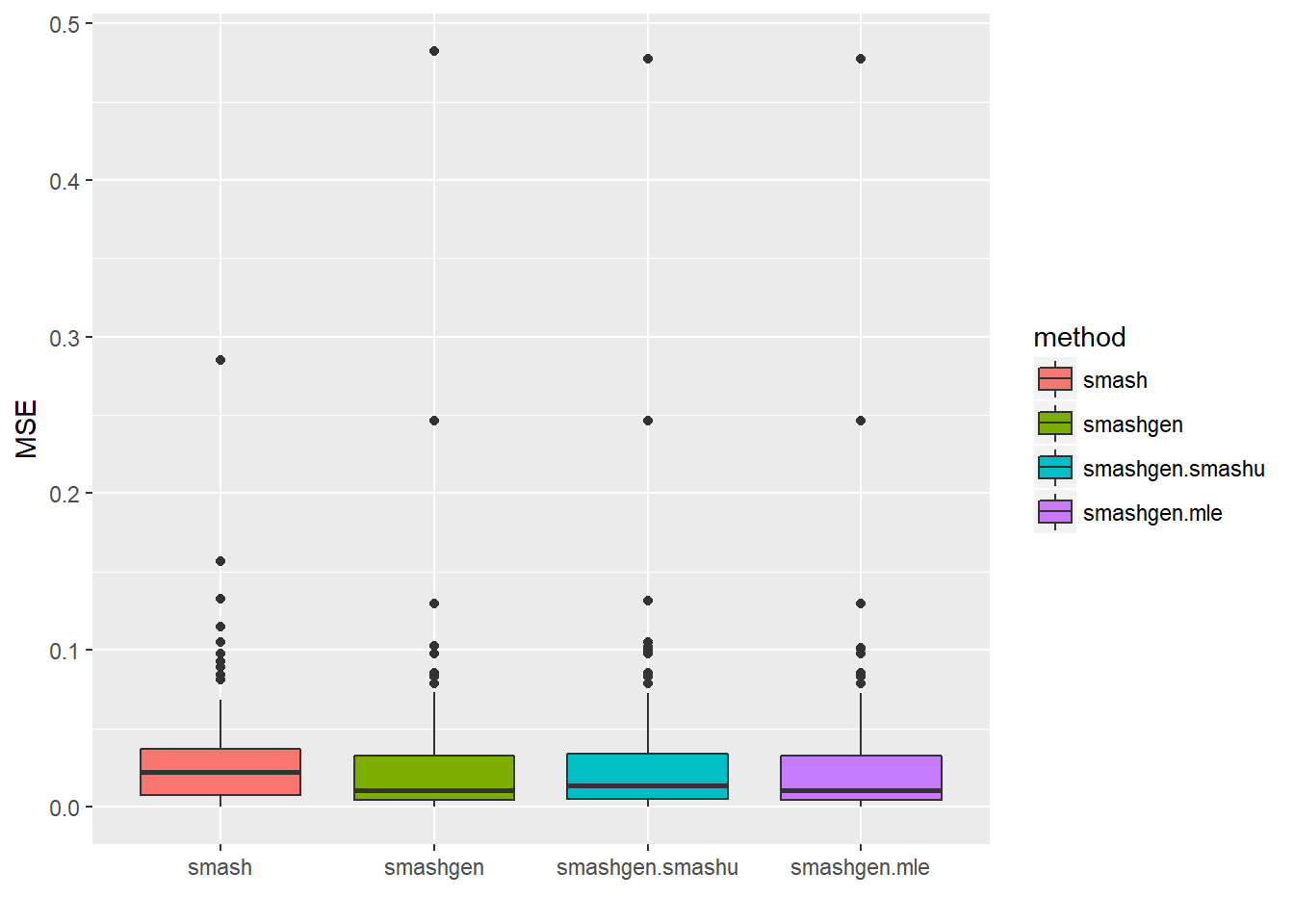
Expand here to see past versions of unnamed-chunk-3-2.png:
| Version | Author | Date |
|---|---|---|
| 594edf1 | Dongyue | 2018-05-17 |
\(\sigma=1\)
m=rep(1,128)
result=simu_study(m,1)
par(mfrow=c(2,2))
plot(result$est$x,col='gray80',ylab='',main='smash')
lines(exp(m),col=1)
lines(result$est$smash.out,col=4)
plot(result$est$x,col='gray80',ylab='',main='smashgen: known sigma')
lines(exp(m),col=1)
lines(result$est$smashgen.out,col=4)
plot(result$est$x,col='gray80',ylab='',main='smashgen: (sigma^2+s_t^2) from smash')
lines(exp(m),col=1)
lines(result$est$smashu.out,col=4)
plot(result$est$x,col='gray80',ylab='',main='smashgen: sigma from mle')
lines(exp(m),col=1)
lines(result$est$mle.out,col=4)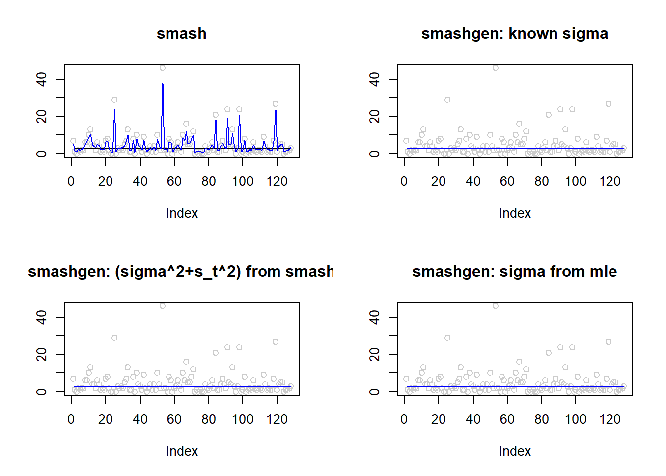
Expand here to see past versions of unnamed-chunk-4-1.png:
| Version | Author | Date |
|---|---|---|
| 594edf1 | Dongyue | 2018-05-17 |
round(apply(result$err,2,mean),4) smash smashgen smashgen.smashu smashgen.mle
29.7351 0.2339 0.2236 0.2884 #ggplot(df2gg(result$err),aes(x=method,y=MSE))+geom_boxplot(aes(fill=method))+labs(x='')\(\sigma=2\)
m=rep(1,128)
result=simu_study(m,2)
par(mfrow=c(2,2))
plot(result$est$x,col='gray80',ylab='',main='smash')
lines(exp(m),col=1)
lines(result$est$smash.out,col=4)
plot(result$est$x,col='gray80',ylab='',main='smashgen: known sigma')
lines(exp(m),col=1)
lines(result$est$smashgen.out,col=4)
plot(result$est$x,col='gray80',ylab='',main='smashgen: (sigma^2+s_t^2) from smash')
lines(exp(m),col=1)
lines(result$est$smashu.out,col=4)
plot(result$est$x,col='gray80',ylab='',main='smashgen: sigma from mle')
lines(exp(m),col=1)
lines(result$est$mle.out,col=4)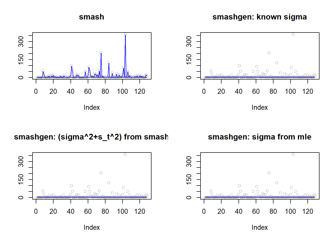
Expand here to see past versions of unnamed-chunk-5-1.png:
| Version | Author | Date |
|---|---|---|
| 594edf1 | Dongyue | 2018-05-17 |
round(apply(result$err,2,mean),4) smash smashgen smashgen.smashu smashgen.mle
8372.2699 0.4992 0.5851 0.5626 #ggplot(df2gg(result$err),aes(x=method,y=MSE))+geom_boxplot(aes(fill=method))+labs(x='')Simulation 2: Step trend
\(\sigma=0.1\)
m=c(rep(3,128), rep(5, 128), rep(6, 128), rep(3, 128))
result=simu_study(m,0.1)
par(mfrow=c(2,2))
plot(result$est$x,col='gray80',ylab='',main='smash')
lines(exp(m),col=1)
lines(result$est$smash.out,col=4)
plot(result$est$x,col='gray80',ylab='',main='smashgen: known sigma')
lines(exp(m),col=1)
lines(result$est$smashgen.out,col=4)
plot(result$est$x,col='gray80',ylab='',main='smashgen: (sigma^2+s_t^2) from smash')
lines(exp(m),col=1)
lines(result$est$smashu.out,col=4)
plot(result$est$x,col='gray80',ylab='',main='smashgen: sigma from mle')
lines(exp(m),col=1)
lines(result$est$mle.out,col=4)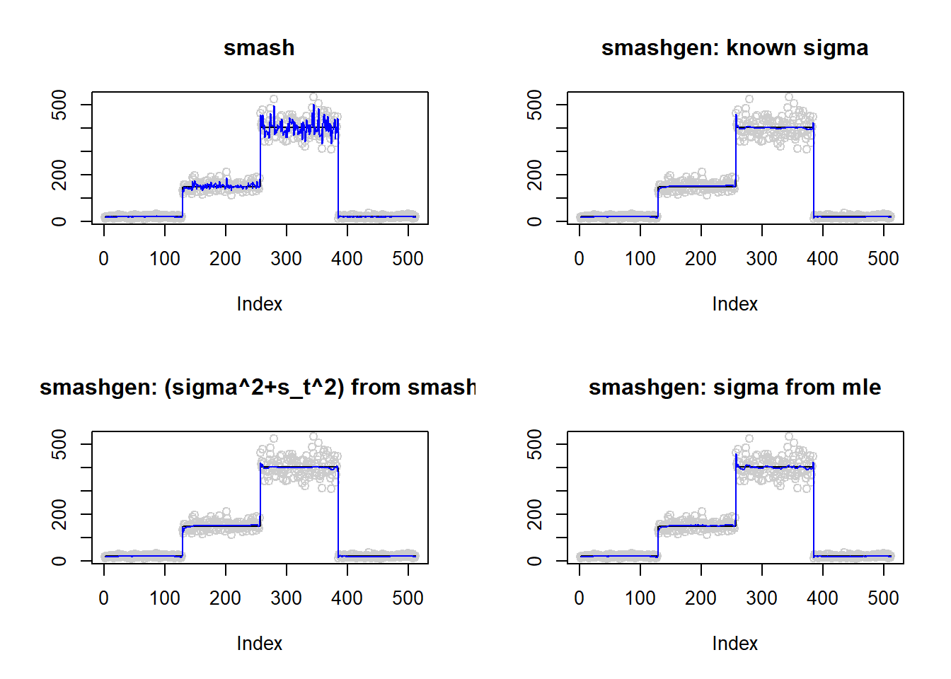
Expand here to see past versions of unnamed-chunk-6-1.png:
| Version | Author | Date |
|---|---|---|
| 594edf1 | Dongyue | 2018-05-17 |
round(apply(result$err,2,mean),4) smash smashgen smashgen.smashu smashgen.mle
368.4722 29.2009 31.9006 36.4252 #ggplot(df2gg(result$err),aes(x=method,y=MSE))+geom_boxplot(aes(fill=method))+labs(x='')\(\sigma=1\)
m=c(rep(3,128), rep(5, 128), rep(6, 128), rep(3, 128))
result=simu_study(m,1)
par(mfrow=c(2,2))
plot(result$est$x,col='gray80',ylab='',main='smash')
lines(exp(m),col=1)
lines(result$est$smash.out,col=4)
plot(result$est$x,col='gray80',ylab='',main='smashgen: known sigma')
lines(exp(m),col=1)
lines(result$est$smashgen.out,col=4)
plot(result$est$x,col='gray80',ylab='',main='smashgen: (sigma^2+s_t^2) from smash')
lines(exp(m),col=1)
lines(result$est$smashu.out,col=4)
plot(result$est$x,col='gray80',ylab='',main='smashgen: sigma from mle')
lines(exp(m),col=1)
lines(result$est$mle.out,col=4)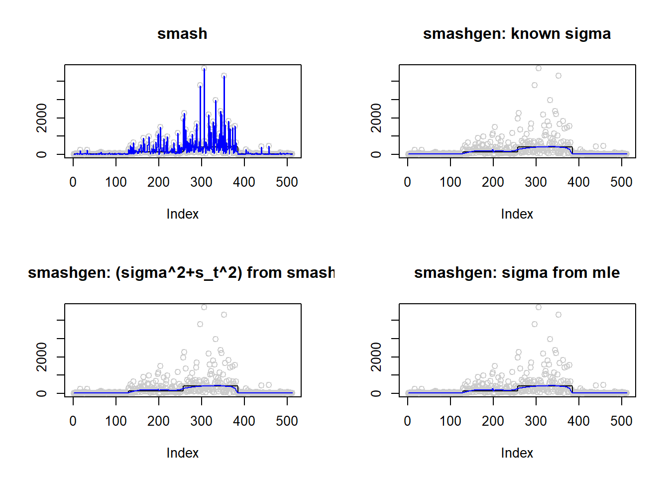
Expand here to see past versions of unnamed-chunk-7-1.png:
| Version | Author | Date |
|---|---|---|
| 594edf1 | Dongyue | 2018-05-17 |
round(apply(result$err,2,mean),4) smash smashgen smashgen.smashu smashgen.mle
223491.625 1658.668 1650.308 1660.029 #ggplot(df2gg(result$err),aes(x=method,y=MSE))+geom_boxplot(aes(fill=method))+labs(x='')Simulation 3: Bumps
\(\sigma=0.1\)
m=seq(0,1,length.out = 256)
h = c(4, 5, 3, 4, 5, 4.2, 2.1, 4.3, 3.1, 5.1, 4.2)
w = c(0.005, 0.005, 0.006, 0.01, 0.01, 0.03, 0.01, 0.01, 0.005,0.008,0.005)
t=c(.1,.13,.15,.23,.25,.4,.44,.65,.76,.78,.81)
f = c()
for(i in 1:length(m)){
  f[i]=sum(h*(1+((m[i]-t)/w)^4)^(-1))
}
m=f
result=simu_study(m,0.1)
par(mfrow=c(2,2))
plot(result$est$x,col='gray80',ylab='',main='smash')
lines(exp(m),col=1)
lines(result$est$smash.out,col=4)
plot(result$est$x,col='gray80',ylab='',main='smashgen: known sigma')
lines(exp(m),col=1)
lines(result$est$smashgen.out,col=4)
plot(result$est$x,col='gray80',ylab='',main='smashgen: (sigma^2+s_t^2) from smash')
lines(exp(m),col=1)
lines(result$est$smashu.out,col=4)
plot(result$est$x,col='gray80',ylab='',main='smashgen: sigma from mle')
lines(exp(m),col=1)
lines(result$est$mle.out,col=4)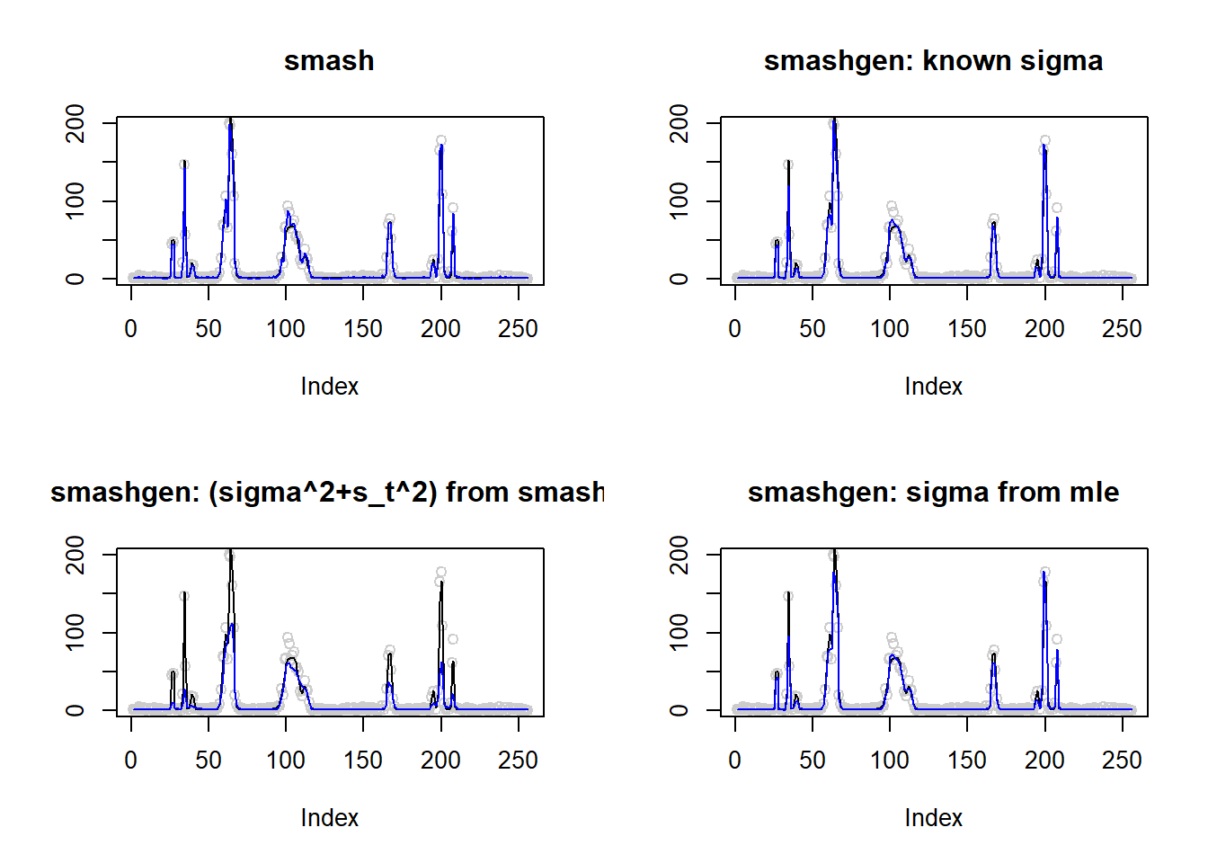
Expand here to see past versions of unnamed-chunk-8-1.png:
| Version | Author | Date |
|---|---|---|
| 594edf1 | Dongyue | 2018-05-17 |
round(apply(result$err,2,mean),4) smash smashgen smashgen.smashu smashgen.mle
23.2597 35.1707 276.9639 36.6836 #ggplot(df2gg(result$err),aes(x=method,y=MSE))+geom_boxplot(aes(fill=method))+labs(x='')\(\sigma=1\)
result=simu_study(m,1)
par(mfrow=c(2,2))
plot(result$est$x,col='gray80',ylab='',main='smash')
lines(exp(m),col=1)
lines(result$est$smash.out,col=4)
plot(result$est$x,col='gray80',ylab='',main='smashgen: known sigma')
lines(exp(m),col=1)
lines(result$est$smashgen.out,col=4)
plot(result$est$x,col='gray80',ylab='',main='smashgen: (sigma^2+s_t^2) from smash')
lines(exp(m),col=1)
lines(result$est$smashu.out,col=4)
plot(result$est$x,col='gray80',ylab='',main='smashgen: sigma from mle')
lines(exp(m),col=1)
lines(result$est$mle.out,col=4)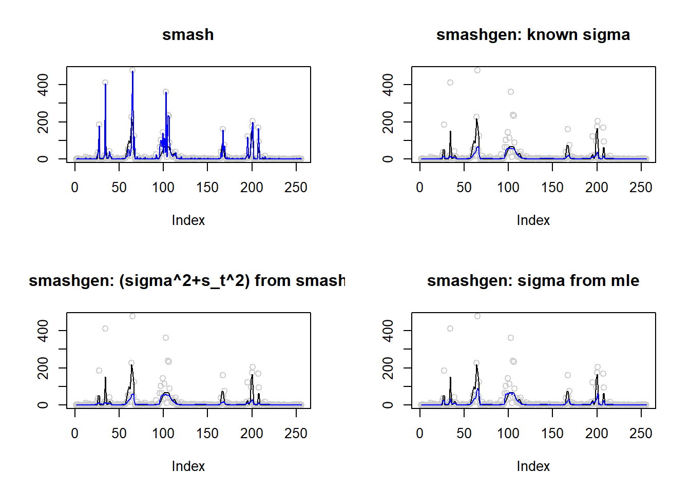
Expand here to see past versions of unnamed-chunk-9-1.png:
| Version | Author | Date |
|---|---|---|
| 594edf1 | Dongyue | 2018-05-17 |
round(apply(result$err,2,mean),4) smash smashgen smashgen.smashu smashgen.mle
6462.4945 480.1025 471.4280 856.6609 #ggplot(df2gg(result$err),aes(x=method,y=MSE))+geom_boxplot(aes(fill=method))+labs(x='')Simulation 4: Doppler
\(\sigma=0.1\)
Small range of \(\mu\)
\(\mu\) in around \((0.1,3.6)\).
m=DJ.EX(256,signal = 1)$doppler
m=log(m-min(m)+0.1)
range(exp(m))
[1] 0.100000 3.565205result=simu_study(m,0.1)
par(mfrow=c(2,2))
plot(result$est$x,col='gray80',ylab='',main='smash')
lines(exp(m),col=1)
lines(result$est$smash.out,col=4)
plot(result$est$x,col='gray80',ylab='',main='smashgen: known sigma')
lines(exp(m),col=1)
lines(result$est$smashgen.out,col=4)
plot(result$est$x,col='gray80',ylab='',main='smashgen: (sigma^2+s_t^2) from smash')
lines(exp(m),col=1)
lines(result$est$smashu.out,col=4)
plot(result$est$x,col='gray80',ylab='',main='smashgen: sigma from mle')
lines(exp(m),col=1)
lines(result$est$mle.out,col=4)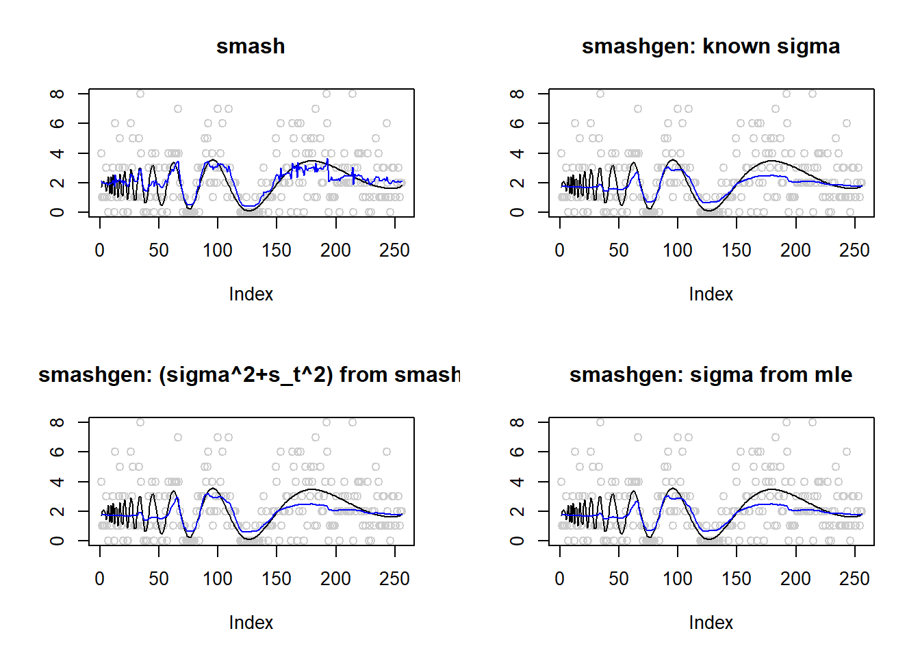
Expand here to see past versions of unnamed-chunk-10-1.png:
| Version | Author | Date |
|---|---|---|
| 594edf1 | Dongyue | 2018-05-17 |
round(apply(result$err,2,mean),4) smash smashgen smashgen.smashu smashgen.mle
0.2596 0.3996 0.3716 0.4022 ggplot(df2gg(result$err),aes(x=method,y=MSE))+geom_boxplot(aes(fill=method))+labs(x='')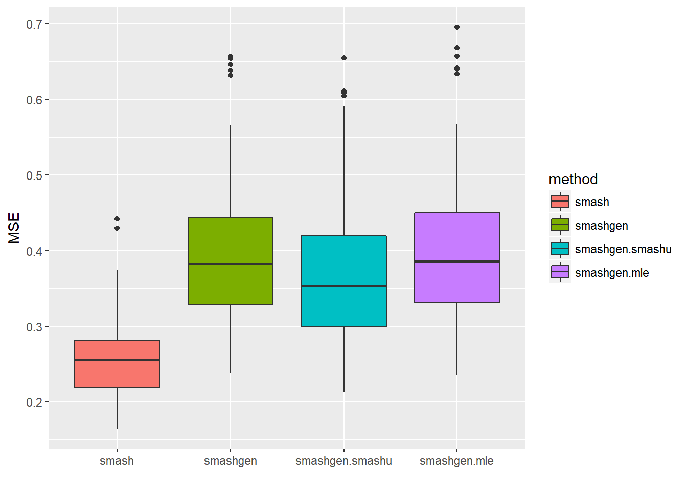
Large range of \(\mu\)
\(\mu\) in around \((0.1,70)\).
m=DJ.EX(256,signal = 20)$doppler
m=log(m-min(m)+0.1)
range(exp(m))
[1] 0.10000 69.40411result=simu_study(m,0.1)
par(mfrow=c(2,2))
plot(result$est$x,col='gray80',ylab='',main='smash')
lines(exp(m),col=1)
lines(result$est$smash.out,col=4)
plot(result$est$x,col='gray80',ylab='',main='smashgen: known sigma')
lines(exp(m),col=1)
lines(result$est$smashgen.out,col=4)
plot(result$est$x,col='gray80',ylab='',main='smashgen: (sigma^2+s_t^2) from smash')
lines(exp(m),col=1)
lines(result$est$smashu.out,col=4)
plot(result$est$x,col='gray80',ylab='',main='smashgen: sigma from mle')
lines(exp(m),col=1)
lines(result$est$mle.out,col=4)
Expand here to see past versions of unnamed-chunk-11-1.png:
| Version | Author | Date |
|---|---|---|
| 594edf1 | Dongyue | 2018-05-17 |
round(apply(result$err,2,mean),4) smash smashgen smashgen.smashu smashgen.mle
26.4471 19.4918 30.7811 20.0644 ggplot(df2gg(result$err),aes(x=method,y=MSE))+geom_boxplot(aes(fill=method))+labs(x='')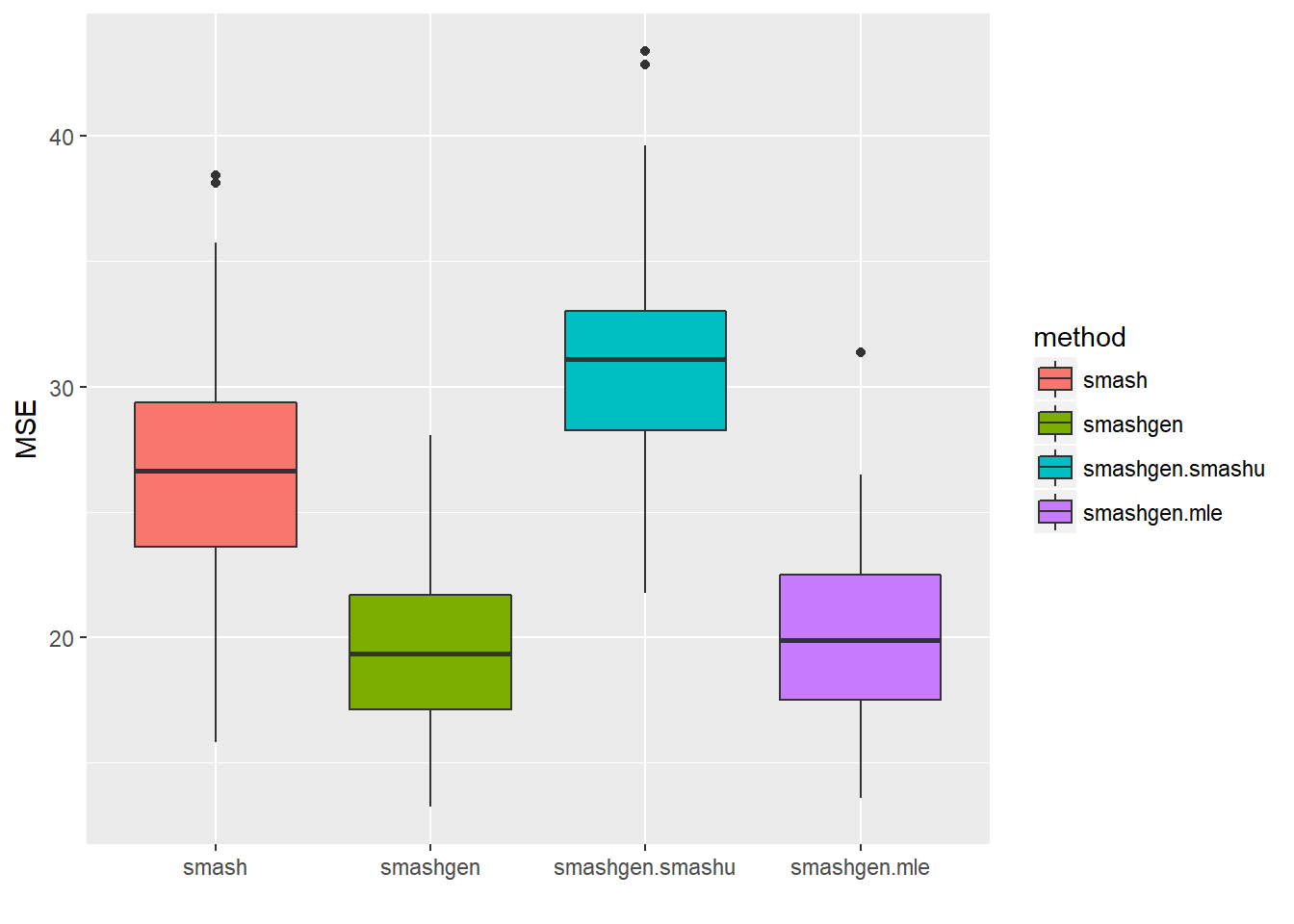
\(\sigma=1\)
Small range of \(\mu\)
\(\mu\) in around \((0.1,3.6)\).
m=DJ.EX(256,signal = 1)$doppler
m=log(m-min(m)+0.1)
range(exp(m))
[1] 0.100000 3.565205result=simu_study(m,1)
par(mfrow=c(2,2))
plot(result$est$x,col='gray80',ylab='',main='smash')
lines(exp(m),col=1)
lines(result$est$smash.out,col=4)
plot(result$est$x,col='gray80',ylab='',main='smashgen: known sigma')
lines(exp(m),col=1)
lines(result$est$smashgen.out,col=4)
plot(result$est$x,col='gray80',ylab='',main='smashgen: (sigma^2+s_t^2) from smash')
lines(exp(m),col=1)
lines(result$est$smashu.out,col=4)
plot(result$est$x,col='gray80',ylab='',main='smashgen: sigma from mle')
lines(exp(m),col=1)
lines(result$est$mle.out,col=4)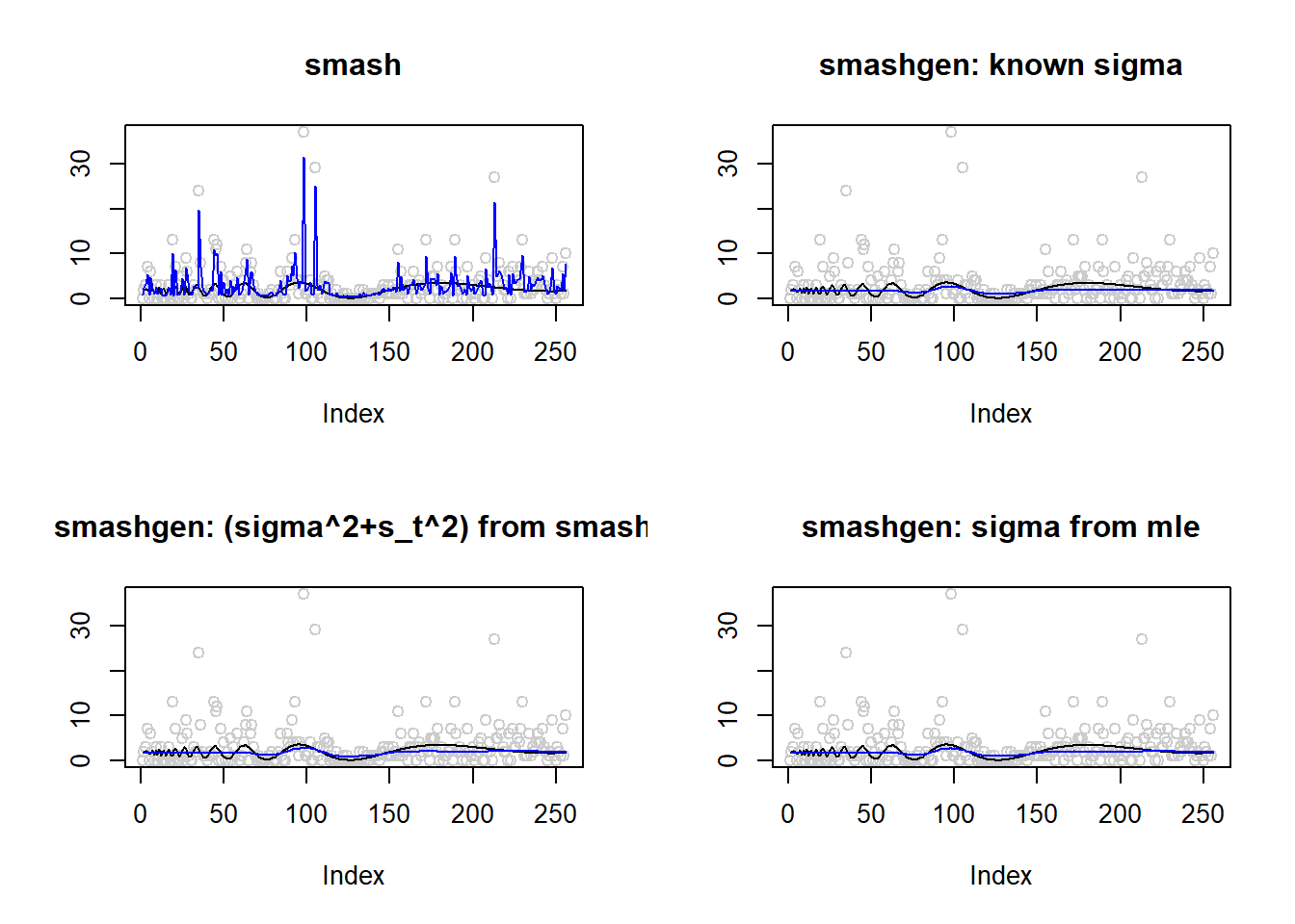
round(apply(result$err,2,mean),4) smash smashgen smashgen.smashu smashgen.mle
2.053750e+01 2.449446e+06 4.712080e+05 1.169379e+07 ggplot(df2gg(result$err),aes(x=method,y=MSE))+geom_boxplot(aes(fill=method))+labs(x='')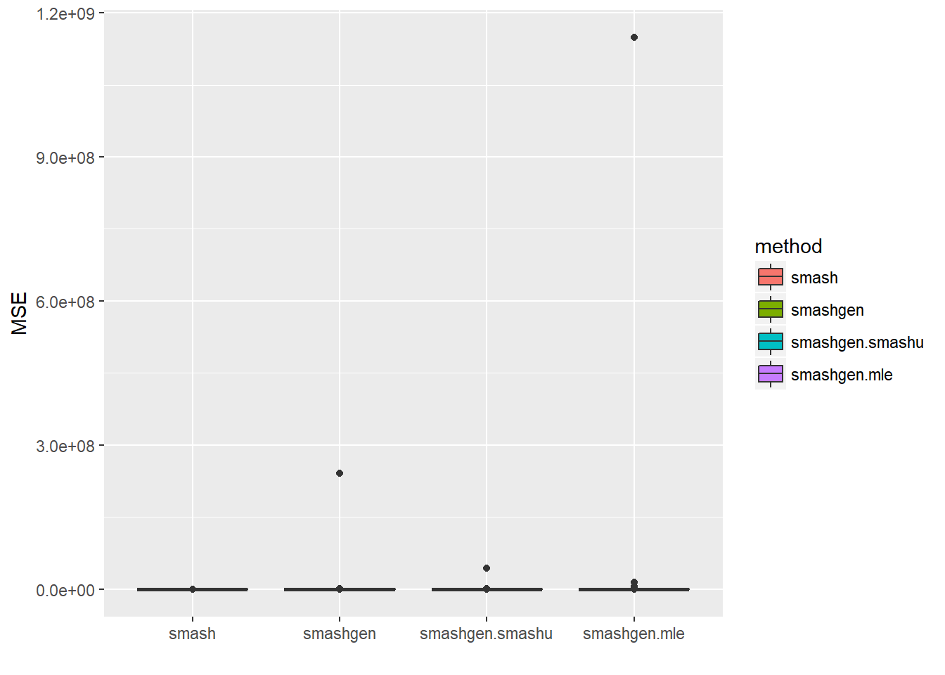
Large range of \(\mu\)
\(\mu\) in around \((0.1,70)\).
m=DJ.EX(256,signal = 20)$doppler
m=log(m-min(m)+0.1)
range(exp(m))
[1] 0.10000 69.40411result=simu_study(m,1)
par(mfrow=c(2,2))
plot(result$est$x,col='gray80',ylab='',main='smash')
lines(exp(m),col=1)
lines(result$est$smash.out,col=4)
plot(result$est$x,col='gray80',ylab='',main='smashgen: known sigma')
lines(exp(m),col=1)
lines(result$est$smashgen.out,col=4)
plot(result$est$x,col='gray80',ylab='',main='smashgen: (sigma^2+s_t^2) from smash')
lines(exp(m),col=1)
lines(result$est$smashu.out,col=4)
plot(result$est$x,col='gray80',ylab='',main='smashgen: sigma from mle')
lines(exp(m),col=1)
lines(result$est$mle.out,col=4)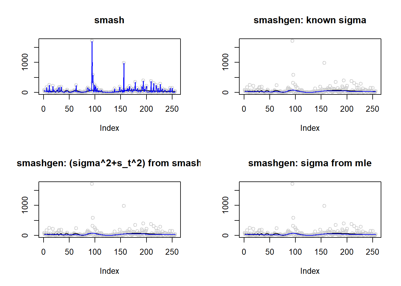
round(apply(result$err,2,mean),4) smash smashgen smashgen.smashu smashgen.mle
9545.5716 131.5410 138.5879 132.0084 ggplot(df2gg(result$err),aes(x=method,y=MSE))+geom_boxplot(aes(fill=method))+labs(x='')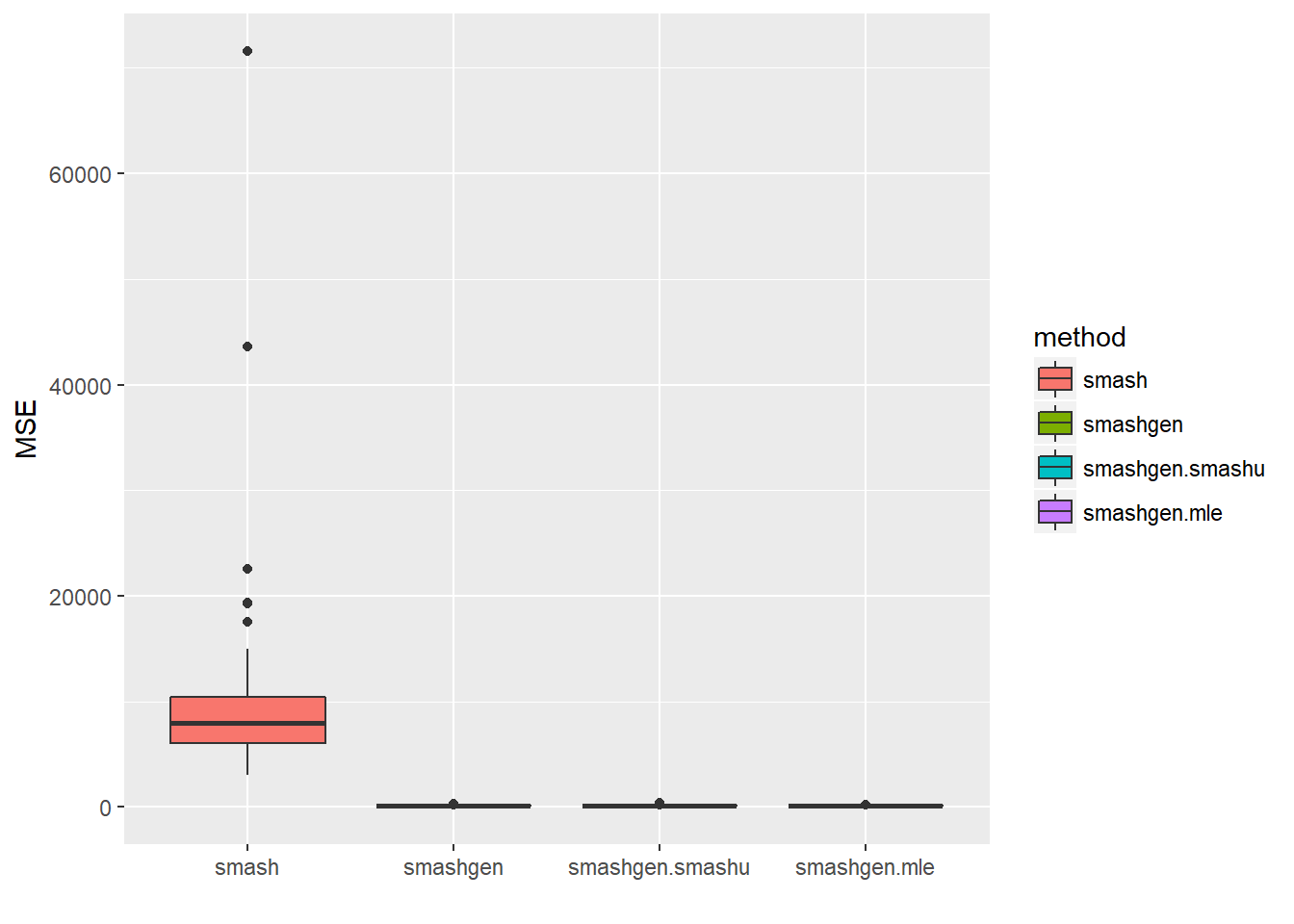
Simulation 5: Spike mean
\(\sigma=0.1\)
Small range of \(\mu\)
\(\mu\) in around \((0.1,6)\).
spike.f = function(x) (0.75 * exp(-500 * (x - 0.23)^2) + 1.5 * exp(-2000 * (x - 0.33)^2) + 3 * exp(-8000 * (x - 0.47)^2) + 2.25 * exp(-16000 *
    (x - 0.69)^2) + 0.5 * exp(-32000 * (x - 0.83)^2))
n = 256
t = 1:n/n
m = spike.f(t)

m=m*2+0.1
m=log(m)
range(exp(m))
[1] 0.100000 6.025467result=simu_study(m,0.1)
par(mfrow=c(2,2))
plot(result$est$x,col='gray80',ylab='',main='smash')
lines(exp(m),col=1)
lines(result$est$smash.out,col=4)
plot(result$est$x,col='gray80',ylab='',main='smashgen: known sigma')
lines(exp(m),col=1)
lines(result$est$smashgen.out,col=4)
plot(result$est$x,col='gray80',ylab='',main='smashgen: (sigma^2+s_t^2) from smash')
lines(exp(m),col=1)
lines(result$est$smashu.out,col=4)
plot(result$est$x,col='gray80',ylab='',main='smashgen: sigma from mle')
lines(exp(m),col=1)
lines(result$est$mle.out,col=4)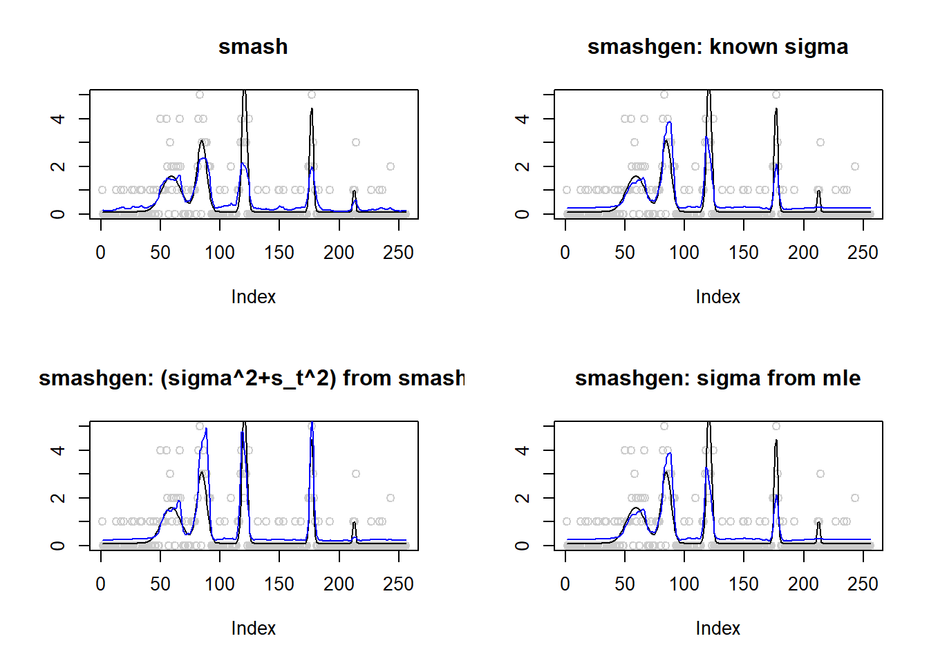
round(apply(result$err,2,mean),4) smash smashgen smashgen.smashu smashgen.mle
0.173 28345959.626 426017.822 28731128.430 ggplot(df2gg(result$err),aes(x=method,y=MSE))+geom_boxplot(aes(fill=method))+labs(x='')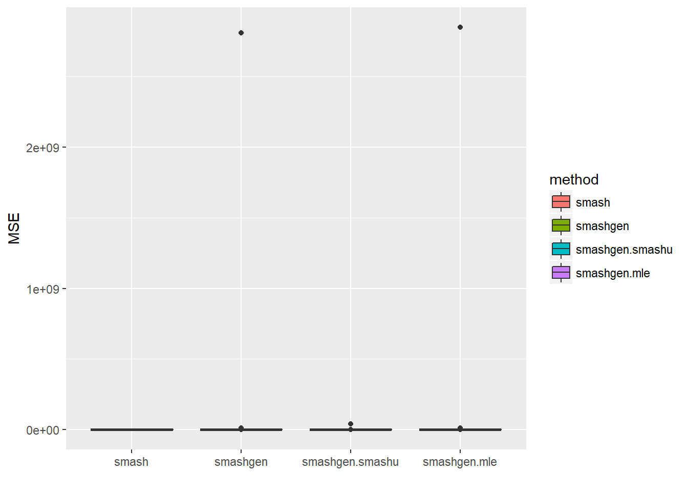
Large range of \(\mu\)
\(\mu\) in around \((0.1,60)\).
spike.f = function(x) (0.75 * exp(-500 * (x - 0.23)^2) + 1.5 * exp(-2000 * (x - 0.33)^2) + 3 * exp(-8000 * (x - 0.47)^2) + 2.25 * exp(-16000 *
    (x - 0.69)^2) + 0.5 * exp(-32000 * (x - 0.83)^2))
n = 256
t = 1:n/n
m = spike.f(t)

m=m*20+0.1
m=log(m)
range(exp(m))
[1] 0.10000 59.35467result=simu_study(m,0.1)
par(mfrow=c(2,2))
plot(result$est$x,col='gray80',ylab='',main='smash')
lines(exp(m),col=1)
lines(result$est$smash.out,col=4)
plot(result$est$x,col='gray80',ylab='',main='smashgen: known sigma')
lines(exp(m),col=1)
lines(result$est$smashgen.out,col=4)
plot(result$est$x,col='gray80',ylab='',main='smashgen: (sigma^2+s_t^2) from smash')
lines(exp(m),col=1)
lines(result$est$smashu.out,col=4)
plot(result$est$x,col='gray80',ylab='',main='smashgen: sigma from mle')
lines(exp(m),col=1)
lines(result$est$mle.out,col=4)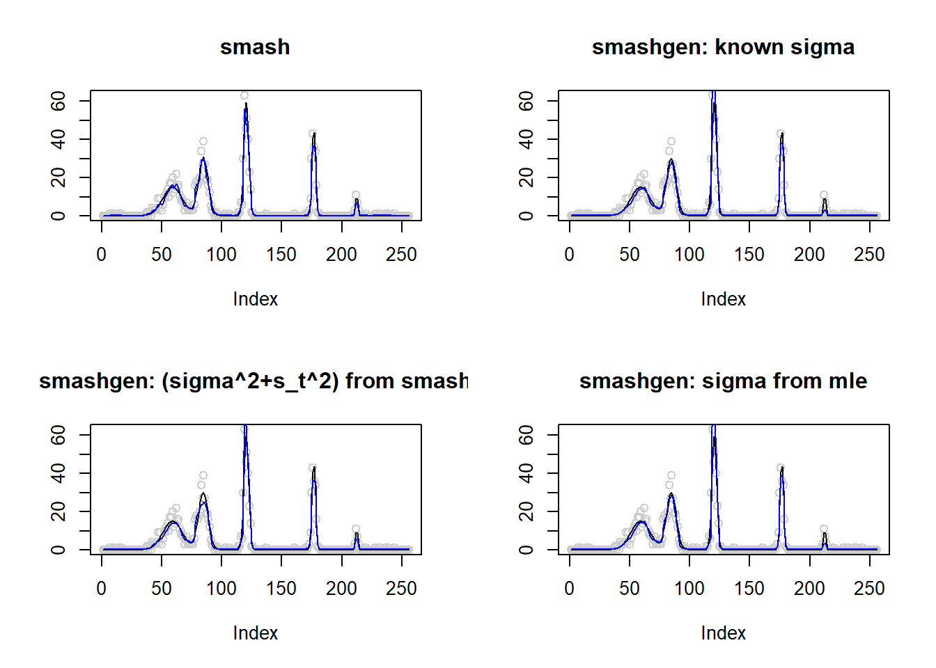
round(apply(result$err,2,mean),4) smash smashgen smashgen.smashu smashgen.mle
3.3231 22.6070 7.3361 26.9417 ggplot(df2gg(result$err),aes(x=method,y=MSE))+geom_boxplot(aes(fill=method))+labs(x='')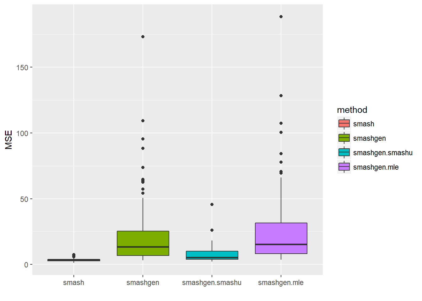
\(\sigma=1\)
Small range of \(\mu\)
\(\mu\) in around \((0.1,6)\).
spike.f = function(x) (0.75 * exp(-500 * (x - 0.23)^2) + 1.5 * exp(-2000 * (x - 0.33)^2) + 3 * exp(-8000 * (x - 0.47)^2) + 2.25 * exp(-16000 *
    (x - 0.69)^2) + 0.5 * exp(-32000 * (x - 0.83)^2))
n = 256
t = 1:n/n
m = spike.f(t)

m=m*2+0.1
m=log(m)
range(exp(m))
[1] 0.100000 6.025467result=simu_study(m,1)
par(mfrow=c(2,2))
plot(result$est$x,col='gray80',ylab='',main='smash')
lines(exp(m),col=1)
lines(result$est$smash.out,col=4)
plot(result$est$x,col='gray80',ylab='',main='smashgen: known sigma')
lines(exp(m),col=1)
lines(result$est$smashgen.out,col=4)
plot(result$est$x,col='gray80',ylab='',main='smashgen: (sigma^2+s_t^2) from smash')
lines(exp(m),col=1)
lines(result$est$smashu.out,col=4)
plot(result$est$x,col='gray80',ylab='',main='smashgen: sigma from mle')
lines(exp(m),col=1)
lines(result$est$mle.out,col=4)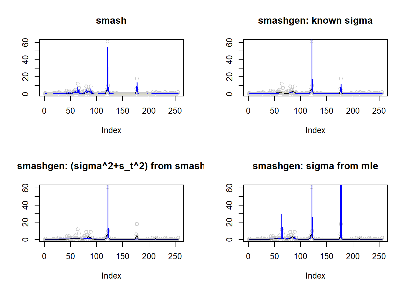
round(apply(result$err,2,mean),4) smash smashgen smashgen.smashu smashgen.mle
4.853800e+00 1.250056e+31 4.210894e+29 1.563109e+31 ggplot(df2gg(result$err),aes(x=method,y=MSE))+geom_boxplot(aes(fill=method))+labs(x='')
Large range of \(\mu\)
\(\mu\) in around \((0.1,60)\).
spike.f = function(x) (0.75 * exp(-500 * (x - 0.23)^2) + 1.5 * exp(-2000 * (x - 0.33)^2) + 3 * exp(-8000 * (x - 0.47)^2) + 2.25 * exp(-16000 *
    (x - 0.69)^2) + 0.5 * exp(-32000 * (x - 0.83)^2))
n = 256
t = 1:n/n
m = spike.f(t)

m=m*20+0.1
m=log(m)
range(exp(m))
[1] 0.10000 59.35467result=simu_study(m,1)
par(mfrow=c(2,2))
plot(result$est$x,col='gray80',ylab='',main='smash')
lines(exp(m),col=1)
lines(result$est$smash.out,col=4)
plot(result$est$x,col='gray80',ylab='',main='smashgen: known sigma')
lines(exp(m),col=1)
lines(result$est$smashgen.out,col=4)
plot(result$est$x,col='gray80',ylab='',main='smashgen: (sigma^2+s_t^2) from smash')
lines(exp(m),col=1)
lines(result$est$smashu.out,col=4)
plot(result$est$x,col='gray80',ylab='',main='smashgen: sigma from mle')
lines(exp(m),col=1)
lines(result$est$mle.out,col=4)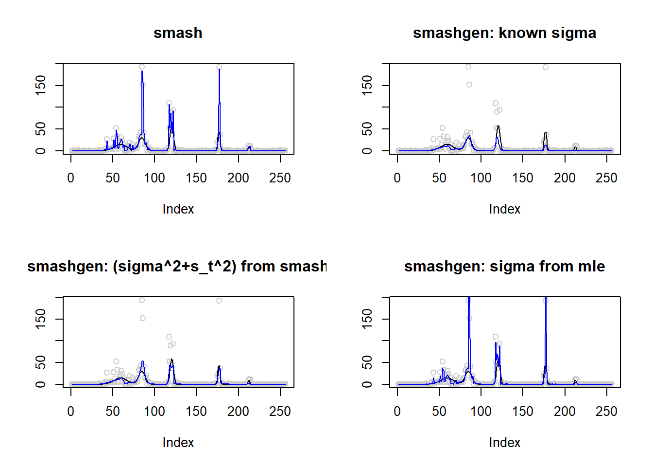
round(apply(result$err,2,mean),4) smash smashgen smashgen.smashu smashgen.mle
704.7864 32.2910 48.5103 1280.0942 ggplot(df2gg(result$err),aes(x=method,y=MSE))+geom_boxplot(aes(fill=method))+labs(x='')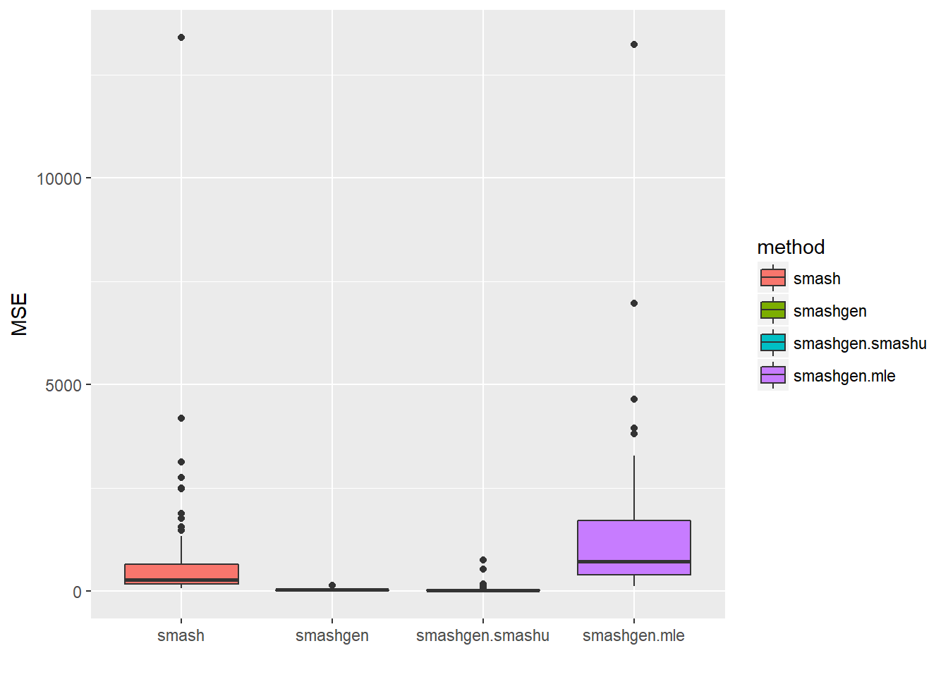
The performance of smashgen is worse than smash.pois for spike mean, especialy when the range of \(\mu\) is small. Smashgen cannot capture the spikes properly which results in huge squared errors. The smash.pois could capture the spikes and it gives noisy fit for the low mean area so it’s MSE is much smaller. Let’s figure out the reason.
One possible reason that causes the issue is that smashgen gives very large fit to the spikes.
Plots of smashgen smoothed wavelets. Blue curves are from smashgen and the black ones are truth.
spike.f = function(x) (0.75 * exp(-500 * (x - 0.23)^2) + 1.5 * exp(-2000 * (x - 0.33)^2) + 3 * exp(-8000 * (x - 0.47)^2) + 2.25 * exp(-16000 *
    (x - 0.69)^2) + 0.5 * exp(-32000 * (x - 0.83)^2))
n = 256
t = 1:n/n
m = spike.f(t)

m=m*2+0.1
m=log(m)

result=simu_study(m,1,nsimu = 6,return.x = T)
par(mfrow=c(3,2))
plot(result$est$x[1,],col='gray80')
lines(exp(m),col='gray30')
lines(result$est$smashgen.smashu.out[1,],col=4)

plot(result$est$x[2,],col='gray80')
lines(exp(m),col='gray30')
lines(result$est$smashgen.smashu.out[2,],col=4)

plot(result$est$x[3,],col='gray80')
lines(exp(m),col='gray30')
lines(result$est$smashgen.smashu.out[3,],col=4)

plot(result$est$x[4,],col='gray80')
lines(exp(m),col='gray30')
lines(result$est$smashgen.smashu.out[4,],col=4)

plot(result$est$x[5,],col='gray80')
lines(exp(m),col='gray30')
lines(result$est$smashgen.smashu.out[5,],col=4)

plot(result$est$x[6,],col='gray80')
lines(exp(m),col='gray30')
lines(result$est$smashgen.smashu.out[6,],col=4)
Larger range of \(\mu\).
m = spike.f(t)

m=m*20+0.1
m=log(m)

result=simu_study(m,1,nsimu = 6,return.x = T)
par(mfrow=c(3,2))
plot(result$est$x[1,],col='gray80')
lines(exp(m),col='gray30')
lines(result$est$smashgen.smashu.out[1,],col=4)

plot(result$est$x[2,],col='gray80')
lines(exp(m),col='gray30')
lines(result$est$smashgen.smashu.out[2,],col=4)

plot(result$est$x[3,],col='gray80')
lines(exp(m),col='gray30')
lines(result$est$smashgen.smashu.out[3,],col=4)

plot(result$est$x[4,],col='gray80')
lines(exp(m),col='gray30')
lines(result$est$smashgen.smashu.out[4,],col=4)

plot(result$est$x[5,],col='gray80')
lines(exp(m),col='gray30')
lines(result$est$smashgen.smashu.out[5,],col=4)

plot(result$est$x[6,],col='gray80')
lines(exp(m),col='gray30')
lines(result$est$smashgen.smashu.out[6,],col=4)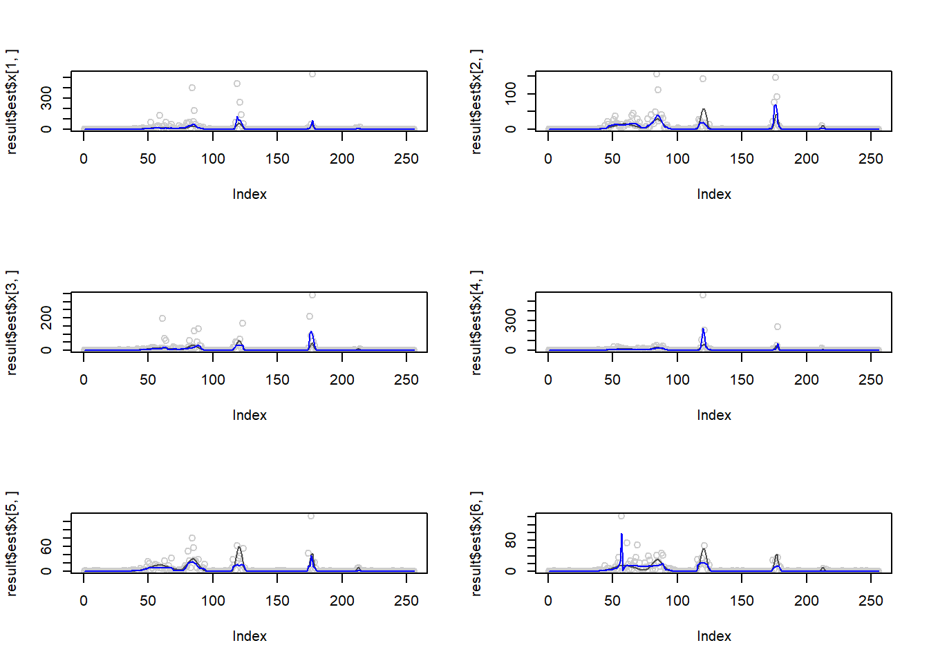
See here for a saperate analysis on this issue.
Session information
sessionInfo()R version 3.4.0 (2017-04-21)
Platform: x86_64-w64-mingw32/x64 (64-bit)
Running under: Windows 10 x64 (build 16299)
Matrix products: default
locale:
[1] LC_COLLATE=English_United States.1252
[2] LC_CTYPE=English_United States.1252
[3] LC_MONETARY=English_United States.1252
[4] LC_NUMERIC=C
[5] LC_TIME=English_United States.1252
attached base packages:
[1] stats graphics grDevices utils datasets methods base
other attached packages:
[1] ggplot2_2.2.1 smashrgen_0.1.0 wavethresh_4.6.8 MASS_7.3-47
[5] caTools_1.17.1 ashr_2.2-7 smashr_1.1-5
loaded via a namespace (and not attached):
[1] Rcpp_0.12.16 plyr_1.8.4 compiler_3.4.0
[4] git2r_0.21.0 workflowr_1.0.1 R.methodsS3_1.7.1
[7] R.utils_2.6.0 bitops_1.0-6 iterators_1.0.8
[10] tools_3.4.0 digest_0.6.13 tibble_1.3.3
[13] evaluate_0.10 gtable_0.2.0 lattice_0.20-35
[16] rlang_0.1.2 Matrix_1.2-9 foreach_1.4.3
[19] yaml_2.1.19 parallel_3.4.0 stringr_1.3.0
[22] knitr_1.20 REBayes_1.3 rprojroot_1.3-2
[25] grid_3.4.0 data.table_1.10.4-3 rmarkdown_1.8
[28] magrittr_1.5 whisker_0.3-2 backports_1.0.5
[31] scales_0.4.1 codetools_0.2-15 htmltools_0.3.5
[34] assertthat_0.2.0 colorspace_1.3-2 labeling_0.3
[37] stringi_1.1.6 Rmosek_8.0.69 lazyeval_0.2.1
[40] munsell_0.4.3 doParallel_1.0.11 pscl_1.4.9
[43] truncnorm_1.0-7 SQUAREM_2017.10-1 R.oo_1.21.0 This reproducible R Markdown analysis was created with workflowr 1.0.1